FINAL REPORT
EARLY IMPLEMENTATION OF NEARSHORE ECOSYSTEM DATABASE PROJECT
Task 3: Review of Procedures, Protocols, Technologies and Providers for Nearshore Marine Habitat Mapping
July 29, 1999
Contractor:
Moss Landing Marine Laboratories
and
California State University, Monterey Bay
via
San Jose State University Foundation Contract # FG 7335 MR
Prepared for:
California Department of Fish and Game
Nearshore Ecosystem Database Project
Compiled by:
Rikk Kvitek, Pat Iampietro, Eric Sandoval, Mike Castleton, Carrie Bretz,
Tally Manouki and Amanda Green
___________
SIVA Resource Center
Institute for Earth Systems Science and Policy
California State University, Monterey Bay100 Campus Center, Seaside, CA 93955
(831) 582-3529
Early Implementation Of The Nearshore Ecosystem Database Project Tasks 2 And 3
1. EXECUTIVE SUMMARY AND RECOMMENDATIONS
*1.1. Background
*1.2. Purpose and Scope
*1.3. Final Products
*1.4. Summary
*1.5. General Findings
*1.6. Recommendations
*2. CONSIDERATIONS FOR EFFECTIVE HABITAT MAPPING
*2.1. Rationale for habitat mapping
*2.2. General approach to habitat mapping
*2.3. Displaying & georeferencing habitat data
*Map scales and data resolution
*Sampling scales
*Map scale and extent
*Coordinate systems, datums and projections
*3. HABITAT CLASSIFICATION SYSTEMS
*3.1. Habitat Classification System proposed by Greene et al.
*Classification of Habitat Scales
*classification structure and terminology
*4. DATA ACQUISITION METHODS
*4.1. Depth and Substrate Data Types
*Bathymetry data
*Seafloor substrate point data
*Seafloor substrate raster data – acoustical methods
*Seafloor substrate raster data – electro-optical methods
*Limitations to acoustic substrate acquisition techniques
*Data acquisition in the very nearshore (0-10 m)
*4.2. Considerations in selecting data acquisition methods
*4.3. Acoustical methods
*Single-beam Bathymetry
*Acoustic Substrate Classifiers
*Multi-Beam Bathymetry
*Sidescan Sonar
*4.4. Electro-optical mapping techniques
*Compact Airborne Spectrographic Imager (CASI)
*LIDAR
*Laser Line Scanner (LLS)
*4.5. Direct 1:1 sampling methods
*Groundtruthing
*Underwater positioning and georeferencing
*5. DATA ACQUISITION TOOLS AND PROVIDERS DATABASE
*5.1. Purpose
*5.2. Methods
*5.3. Results
*5.4. Conclusions
*6. FINAL PRODUCT OPTIONS
*7. EXISTING SEAFLOOR SUBSTRATE DATA CATALOG (NEDP-TASK 2)
*7.1. Introduction
*7.2. Methods
*7.3. Results
*California Dept. of Conservation- Division of Mines and Geology/Moss Landing Marine Labs
*US Geological Survey
*National Geodetic Data Center
*Monterey Bay Aquarium Research Institute
*California State University Monterey Bay
*Ecoscan Resource Data
*Proprietary Data
*Office of Naval Research
*Limitations of the CERES Spatial Metadata Record Template
*Primary sources & pending data
*7.4. Conclusions
*7.5. Recommendations
*8. BIBLIOGRAPHY
*9. ACKNOWLEDGEMENTS
*EXECUTIVE SUMMARY AND RECOMMENDATIONS
The California Department of Fish and Game Nearshore Ecosystem Database Project is designed to address the policy of the State to assess, conserve, restore, and manage California’s ocean resources and the ecosystem as stated in Executive Order No. W-162-97. The purpose of this project is to enable the Department to expand its Geographic Information System (GIS) database to include and make available to CERES, data from the marine subtidal and nearshore ecosystems. The primary components of the project are: GIS mapping of essential marine habitats, nearshore reef fish stock assessment, and marine reserve research. The Early Implementation Phase of this project has focused on accelerating the acquisition of baseline bathymetry and substrate data as outlined in the GIS Mapping of Essential Marine Habitats portion of the project. This effort has included four tasks:
Task 1) Data Needs: Identification of departmental needs for bathymetry and substrate data.
Task 2) Data Catalog: Assessment and collection of metadata for currently available data on marine bathymetry and seafloor substrates.
Task 3) Procedures, Protocols and New Technologies: A review of current and emerging methods and providers for mapping marine habitats.
Task 4) Data Processing: Process and incorporate existing bathymetric and substrate data into Department GIS coverage themes.
The focus of this report is on those portions of Tasks 2 and 3 subcontracted to Moss Landing Marine Laboratories and California State University Monterey Bay through San Jose State University Foundation (Contract # FG 7335 MR). For Task 2, the work was divided, with the Department taking on the collection and assessment of metadata for bathymetry, and this contract covering the metadata for existing substrate information. For Task 3 our assignment was to survey and evaluate currently available techniques for mapping marine habitats, and to assess their adequacy for meeting stated Department data needs. Here our goal has been to provide the Department with the information needed to make decisions on: 1) how habitats of interest should be mapped given the needs of the Department, 2) the selection of providers of marine habitat mapping services and equipment, and 3) the relative costs in time and money associated with acquiring the types of habitat data needed.
The Department requested that we limit our scope to the California continental shelf, giving primary attention to the nearshore 0-30 m depth zone. It is this shallow coastal zone that is often the most heavy utilized and impacted by human activities, yet it is also the zone for which we have the least amount of bathymetric and substrate data. This data scarcity is due in large part to the challenging and often dangerous logistics associated with conducting hydrographic surveys in shallow, open coast environments. High use and data scarcities have made the 0-30 m depth zone a high priority for habitat mapping over the next decade.
Our final products for this project include the written final report and two Microsoft Access databases, one containing information on habitat mapping technologies and providers (Mapping Tools Database), and the other the CERES compliant metadata catalogue for existing seafloor substrate data sets. In the report we review and summarize the reasons for, approaches to and requirements of habitat mapping as they apply to nearshore marine resource management. Also in the report, we review and summarize in tabular form the data contained in the two databases. The Habitat Mapping Tools Database contains information on the Tools, Tool Manufacturers, Survey Equipment Providers, and Survey Service Providers (including private companies, universities and government agencies). The Seafloor Substrate Metadata Catalog contains information on 85 data sets obtained after contacting 86 potential sources.
A habitat is the place where a particular species lives or biotic community is normally found. Habitat mapping is often undertaken by resource agencies to serve a variety of purposes including:
While most subtidal species and resources can only be sampled directly using observational or other large scale (>1:10,000) survey techniques, it would be impractical to apply this level of effort to the entire coast of California. A major goal of habitat mapping, therefore, is to develop the ability to predict the distribution and abundance of species and resources from those physical and biotic parameters that can be remotely sampled.
Habitat parameters important to the distribution and abundance of benthic and nearshore species include but are not limited to: water depth, substrate type, rugosity, slope/aspect, voids (abundance, type and size), sediment type and depth, exposure, vegetation, chemistry, temperature, presence of other species.
Because the response of different species often varies with the spatial extent of these parameters, habitat scale is another factor important in defining where different species and biotic communities are likely to be found. For this reason, a benthic habitat classification system useful for defining species/habitat associations based on the parameters listed above must also be hierarchically organized according to relevant spatial scales.
Given these considerations, a regional habitat mapping program should include the following elements:
There are now keen interests, new legislative mandates, and compelling needs driving many state and federal management agencies in the direction of nearshore habitat mapping. Most agencies, however, lack the expertise, equipment, and financial ability to collect, process, analyze, and use the types of habitat data required by these new mandates. Those that do or did, such as the US Geological Survey, have been faced with the loss of experienced personnel through downsizing, and the fiscal inability to keep up with the rapidly changing and very expensive technologies required. While there are numerous private companies that do have these capabilities, much of their mapping work has been done for private interests (e.g. telecommunications companies) that are either not permitted or willing to share their data with public agencies due to a highly competitive market place. Military data, though potentially abundant regionally, is primarily in hard copy form, poorly georeferenced, and difficult to locate and access without help and interest from within the military.
As a result of these factors, several agencies including the Department of Fish and Game are exploring the avenues open to them for acquiring and utilizing marine habitat data. To date, however, there has been little coordination to leverage these efforts among the interested agencies. Further confounding matters is the lack of a generally accepted habitat classification system appropriate for nearshore marine environments. This lack of coordination means that efforts will be duplicated, and that data sharing will be hampered by lack of uniformity in data collection, classification and processing protocols. Given that marine biotic habitat mapping is still in its infancy, however, there remains an opportunity to coordinate and leverage resources in the development of these habitat maps, technologies and protocols.
The established methods and acoustic mapping technologies in current use are capable of creating highly detailed maps of 3D seafloor morphology and substrate type at sub-meter resolutions over broad areas of habitat. Much of the biotically important detail in habitats, however, can occur at the level of decimeters and centimeters. As a result, direct sampling and video imagery are often necessary to augment the detail provided via acoustic remote sensing. While the combination of these methods is capable of yielding highly detailed results, the expense involved can be impractical due to the relatively slow data acquisition rates compared to that required for remote sensing in terrestrial habitats. Obtaining a high resolution, groundtruthed image of a square kilometer of seafloor can take more than a day to acquire at great expense, compared to just minutes needed to obtain relatively inexpensive aerial photographic coverage of terrestrial habitat. Given the extensive coastline of California and the fact that it is often impossible to conduct conventional boat-based acoustic surveys in the 0-10m depth range due to geohazards, new more efficient mapping technologies need to be developed. Emerging laser and digital video mapping techniques such as LIDAR, Laser linescan and CASI, may enable aircraft to routinely sample the bathymetry and substrate in intertidal and shallow subtidal habitats that are inaccessible or too costly for conventional acoustic survey methods.
Regardless of which type of high resolution, broad coverage seafloor mapping techniques are selected, the cost of the equipment and expertise required to effectively operate and maintain it will generally be outside the budget of most resource management agencies. As a result, most agencies will find it cost effective to contract out for the actual acquisition of seafloor survey data, while developing the more generically useful GIS capabilities in-house that are required for the synthesis, analysis, display and application of these data.
Based on these findings we make the following recommendations to the Department regarding the development of habitat maps for the California nearshore environment.
CONSIDERATIONS FOR EFFECTIVE HABITAT MAPPING
2.1 RATIONALE FOR HABITAT MAPPING
A habitat is the place where a particular species lives or biotic community is normally found, and is often characterized by the dominant life form (e.g. kelp forest habitat) or physical characteristics (e.g. rocky subtidal habitat). Because habitats are repetitive physical or biophysical units found within ecosystems the same habitat may be found within different biogeographical provinces. Habitat mapping is typically undertaken by resource agencies to serve a variety of purposes including:
While most subtidal species and resources can only be sampled directly using observational or other large scale (>1:10,000) survey techniques, it is often unreasonable to apply this level of effort to the entire coast of California. A major goal of habitat mapping, therefore, is to develop the ability to predict the distribution and abundance of species and resources from those physical and biotic parameters that define where species live and which can be remotely sampled.
The geographic limits to the distribution of many marine species result from barriers to migration, reproduction or survival. These biogeographic barriers result in ranges within which a species or community assemblage are likely to occur within the same habitat types. The habitat types can be defined in terms of those variables that control where a species lives within its range. Habitat parameters important to the distribution and abundance of benthic and nearshore species include:
Because the response of different species often varies with the spatial extent of these parameters, habitat scale is another factor important in defining where different species and biotic communities are likely to be found. For this reason, a benthic habitat classification system useful for defining species/habitat associations based on the parameters listed above, must also be hierarchically organized according to relevant spatial scales (see Habitat Classification Systems below).
Given these considerations, a successful, regional habitat mapping program needs to include the following elements:
Each of these elements is discussed in the following sections. In Section 2.2 we give a brief overview of the purposes for and general approach to benthic habitat mapping. We then cover some of the issues pertaining to scale and georeferencing habitat data in Section 2.3. Requirements and recommendations for a suitable benthic habitat classification system are discussed in Section 3. We then review and provide examples from a wide range of habitat data acquisition methods in Section 4, covering the advantages and limitations of standard methods as well as those of emerging new technologies. Information on specifications, manufacturers, and service providers using these data acquisition tools have been compiled into an extensive database, and summarized in tables presented in Section 5.
In our discussion of the types of final product options available for habitat mapping projects in Section 6, we give only a brief overview of the various approaches available for data fusion, analysis and display of habitat data. Recent advances in Geographic Information Systems (GIS) have now brought spatial data analysis and display capabilities to virtually every desk top computer. While we use GIS extensively in our own habitat mapping work, and will make use of several of our GIS products as examples in this report, we will leave the review and assessment of GIS systems and applications to other authors. This decision is consistent with DFG's request that we focus our efforts on reviewing the specific technologies for the acquisition and classification of seafloor substrate and depth data.
2.2 GENERAL APPROACH TO HABITAT MAPPING
In recent years, many marine benthic habitats have been described using biological and geophysical data. Consequently, remote sensing and large-scale mapping of the seafloor are gaining popularity for assessing habitats as well as potential impact of human disturbances (such as bottom trawling) on benthic organisms. Because many benthic habitats are defined by their geology (along with depth, chemistry, associated biotic communities and other attributes), geophysical techniques are critical in determining habitat type. However, with the increased use of multidisciplinary techniques (i.e., in situ observations as well as geophysical sensors) and nomenclature (geological, geophysical and biological) to define benthic habitats, a standard habitat characterization scheme is needed to more accurately and efficiently interpret and compare habitats and associated assemblages across biogeographic regions and among scientific disciplines (Greene et al. in press).
Geophysical techniques that help identify and define large-scale marine benthic features are valuable in appraising essential habitats of marine benthic fish assemblages. Interpretations and verification of sidescan sonar, swath bathymetry, backscatter imagery, and seismic reflection profiles with direct observation and sampling of rock and biogenic fauna are critical in characterizing these habitats. As a result, the adopted classification scheme must be compatible with data collected with all types of sensor systems used to characterize habitats (e.g. acoustic, Electro-optical, optical and direct sampling).
Modern marine geophysical techniques are now being used to investigate and characterize benthic habitats (Able et al., 1987, 1995; Auster et al., 1995; Greene et al., 1993, 1994, 1995; O’Connell and Wakefield, 1995; O’Connell et al., 1997; Twichell and Able, 1993; Yoklavich, 1997; Yoklavich et al, 1992, 1995, 1997; Wakefield et al., 1996; Valentine and Lough, 1991; Valentine and Schmuck, 1995). The most commonly applied remote sensing methods for benthic habitats involve acoustical techniques that use sound sources of different frequencies to produce images of surface and subsurface features of the seafloor. Reflected sound waves are recorded as seafloor images in plane, aerial and cross-section views. Additionally, increased availability and use of underwater video systems on remotely operated vehicles (ROV's), submersibles, and camera sleds have made fine-grained remote sensing surveys of habitats and associated biological assemblages more commonplace, thereby expanding our understanding of the processes that help define these communities and the spatial scale at which these processes operate (Greene et al. in press). Once perfected, emerging new technologies such as LIDAR, CASI and Laser Line Scanners may greatly increase the speed and efficiency of collecting high-resolution habitat data (see Chapter 4 below).
Although habitat characterization pertaining to fish and fisheries is in its infancy, several pioneering studies have been done along the continental margin of North America. Fisheries habitat has been studied in the Gulf of Maine, over the Georges and Stellwagen Banks (Lough et al., 1989, 1992, 1993; Valentine and Lough, 1991; Valentine and Schmuck, 1995), middle Atlantic Bight (Auster et al., 1991), and other areas along the east coast of the US (Able et al., 1987, 1995; Twichell and Able, 1993). Along the west coast of North America recent investigations of benthic habitats of rockfishes have been reported of central California (Greene et al., 1994, 1995; Yoklavich et al., 1992, 1995, 1997), British Columbia (Matthew and Richards, 1991) and in southeast Alaska (O'Connell and Carlile, 1993; O’Connell et al 1997).
2.3 DISPLAYING & GEOREFERENCING HABITAT DATA
There are four key considerations related to the display and georeferencing of habitat data:
Map scales and data resolution
With the advent of geographic information systems (GIS) it is now possible to merge, layer and display virtually all geocoded habitat data at any desired scale. Unfortunately, data collected at one scale may lose its meaning when displayed at a scale that is inappropriate for either the resolution (spatial density) or extent of the data set. Thus, while data collected at a particular resolution within a given area may be adequate for one purpose, it may not be suitable for other habitat mapping needs. For example, polygon features representing habitat classes measuring < 100 m2 within a small coastal marine reserve can be accurately displayed at large map scales (>1:10,000). These same features will shrink to lines, points or disappear entirely on smaller scale maps (< 1:50:000) such as those used for displaying the regional distribution of fisheries or habitats (Table 2.1). Although GIS can circumvent this issue of display scale to some extent by providing the user with the ability to zoom in and out, the utility of hardcopy products are severely effected by the scale of display.
Table 2.1 Standard mapping scales and resulting display resolutions (adapted from Booth et al. 1996, and Greene et al., in press).
|
Scale |
1 mm = (m) |
1 mm2 = (ha or m2) |
Planning Class |
Features that can be displayed at this map scale |
|
1:106 |
1,000 |
100 ha |
Hemisphere |
Megahabitats, Biogeographic regions, species & fisheries range boundaries |
|
1:500,000 |
500 |
25 ha |
Regional |
Megahabitats, Biogeographic zones, gross shoreline features, resource management jurisdictions |
|
1:250,000 |
250 |
6.25 ha |
Sub-regional |
Megahabitats, Geologic mapping, river mouths, bays, estuaries, habitat features, fishing grounds |
|
1:50,000 to 100,000 |
50-100 |
0.25 to 1.00 ha |
Local |
Mesohabitats, Marine reserve boundaries, small islands and inlets, habitat classes |
|
1:24,000 |
24 |
576 m2 |
Local, site |
Mesohabitats, Fine grain habitat mapping, off-shore rocks, kelp beds, substrate type |
|
1:10,000 |
10 |
100 m2 |
Site |
Mesohabitats, High resolution habitat mapping, seabed texture |
|
1:1,000 to 5,000 |
1 - 5 |
1 - 25 m2 |
Site |
Macro- and Microhabitats, Biotic community and site level mapping |
There is also the relationship between map scale and data resolution. While it is possible to collect high-resolution data over vast areas, the cost of doing so, and the size of the resulting data sets may be impractical if the primary purpose is to provide a regional overview of gross habitat types. Consequently, the selection of map scale depends on two factors: 1) the scale of the base map to be used (see below) and 2) the purpose of the study.
Table 2.2 General categories of methods for sampling coastal subtidal habitats and the scales at which they can be used (after Robinson et al. 1996).
|
Sampling scale |
Method |
Examples |
|
1:30,000 |
Satellite sensors |
SPOT, Landsat, AVHRR |
|
1:5,000 to 1:20,000 |
Airborne sensors |
Aerial Video Imagery (AVI) and Aerial Photography (AP) Larsen Airborne Laser Bathymetry (LIDAR) which uses infrared and blue/green laser pulses to measure seafloor depth; possibly other information contained in backscatter characteristics such as fish schools and bottom type Compact Airborne Spectral Imager (CASI): a multispectral sensor that digitally records data along the flight path. |
|
1:10 to 1:10,000 |
Laser line scanner |
Towed or airborne sensor capable of near video quality swath imaging of seafloor |
|
1:1000 to 1:10,000 |
Hydroacoustic sensors and post-processors |
Low frequency echosounders for water depth and with post-processing of return backscatter for substrate characteristics. Sidescan sonar can visualize seafloor morphology and seabed texture |
|
1:10 to 1:1000 |
In situ visual or camera sampling |
Free swimming or towed SCUBA Remotely Operated Vehicles (ROV) Drop or towed cameras |
|
1:10 to 1:100 |
Removal sampling methods |
In situ sampling by divers or ROV’s Remote stationary sampling methods: grab or core samples |
The highest level of a hierarchical classification system that can be applied to an ecosystem will depend on those variables that can be sampled at the smallest scale. This consideration is especially relevant to the California shallow nearshore coastal zone, which is long but very narrow. The high length to width aspect ratio of this zone requires larger sampling scales to provide adequate habitat resolution than is customary in offshore or terrestrial habitat mapping. Otherwise, along shore habitat features will be reduced to lines rather than areas. Booth et al. (1996) point out, however, that there are several large scale variables (e.g. wave height, current velocity, exposure, coastal morphology) that can be derived from smaller scale features such as coastlines on maps drawn at the 1:40,000 to 1:200,000 scale.
Because the way in which a variable is sampled will affect the scale at which it can be meaningfully displayed or classified, it is important to match how habitats are sampled with the overall scale of the project. Robinson et al. (1996) reviewed the sampling methodology presently available for sampling subtidal environments (Table 2.2).
California coastal habitats within the 0 - 30 m depth range exist within a narrow zone often extending no more than a kilometer from shore. As a result, many of the coastal features such as reefs and islands are lost at smaller mapping scales (<1:100,000) and must be mapped and displayed at larger scale.
Mega-habitat mapping scales (< 1:100,000)
The published California Continental Margin maps (Greene and Kennedy 1986) drawn at the 1:250,000 scale, show the major geophysical seafloor features for the California continental shelf. While the sediments and substrate types depicted on these maps are relevant to the classification of marine habitats, the scale at which they are depicted limits their utility within the shallow subtidal. At this scale, habitat elements within the 0-30 m depth range are reduced to line features at best. These maps are nevertheless an excellent reference data set for megahabitat or regional scale habitat mapping, and correspond to the 1:250,000 mapping scale recommended as a standard for mapping coastal resources at the "Provincial" (regional) scale in Booth et al.'s 1996 technical report to Fisheries and Oceans Canada. Larger map scales (>1:50,000), however, are required for mapping and displaying most of the habitat features within the 0-30m depth zone.
Meso-habitat mapping scales (1:100,000 to 10,000)
Even at the larger mapping scale of 1:50,000, important coastal habitat features such as kelp forests, offshore rocks and reefs become reduced to one dimensional line features rather than polygons. More appropriate for nearshore habitat mapping of coastal features is the 1:24,000 scale common to the USGS topographic 7.5 minute quadrangle maps. This scale and set of map boundaries have already been used to provide the base maps for:
At this scale, features down to 24 m in linear dimension can be easily depicted. Given the wide application of the 7.5 minute quad scale and footprint, we recommend its extension to nearshore coastal habitat mapping at the local scale.
Macro- and Micro- habitat mapping scales
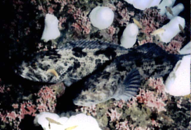
Much of the physical detail important to many species occurs at the meter and sub-meter scale (e.g. substrate texture, grain size, void spacing and size). As a result, data collection and mapping capable of depicting this detail is critical to habitat classification at the Macro- and Micro-habitat scales (Figs. 2.1 and 2.2).
Figure 2.1. Biological microhabitats of hydrocorals and sea anemones with lingcod (Ophiodon elongatus) and young of the year rockfish (Sebastes spp.) on top of rock pinnacle mesohabitat (photo courtesy of Greene et al. in press).
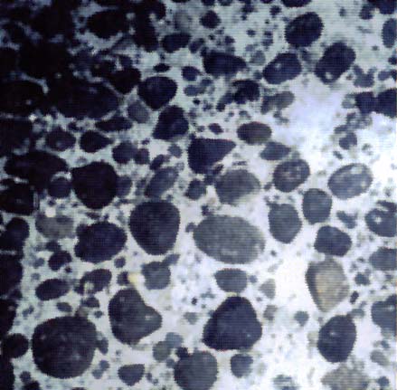
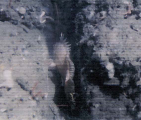
Figure 2.2. Examples of Micro- and Macro-habitats. (Left) Pebble microhabitat in offshore Edgecumbe lava field, southeast Alaska (Greene et al. in press). (Right) Crevice in the Pliocene Purisima Formation that has been differentially eroded along the walls of Soquel Canyon, Monterey Bay, California (photos courtesy of Greene et al. in press).
Coordinate systems, datums and projections
As with scale, GIS can be used to display and merge virtually any geocoded habitat data regardless of the geodetic parameters under which they are collected or archived. For example, vector data collected in latitude and longitude NAD83 can be easily combined with raster imagery registered as UTM WGS 1984 data. However, the importance of selecting and knowing the geodetic parameters of the data sets cannot be over emphasized. First, while most true GIS systems (e.g. ArcInfo, TNT MIPS) are able to process and merge data having different geodetic parameters, this data fusion is only successful when these parameters are correctly defined for the program. If, for example, lat long data collected in California using the North American Datum 1927 (NAD27) is merged with lat long North American Datum 1983 (NAD83) data without specifying the correct datum for each data set, the registration of the two data sets will be off by nearly 100 m in the east/west direction.
Secondly, not all "GIS" type programs are capable of accurately merging data having different geodetic parameters. ArcView, the most popular GIS viewer program, cannot be used to reproject geospatial data. Once an ArcView project file has been created for a specific set of geodetic parameters, only those data sets stored in the same coordinate system, datum and projection as the project file can be accurately added as a theme. Here again, while it may be possible to import data sets having different geodetic parameters into ArcView as themes, they will not be correctly georegistered. ArcView, however, is a rapidly evolving program, and may eventually have the ability to reproject and co-register data from different projections, datums and coordinate systems. Until this capability is added, data will have to be initially collected or reprocessed using a true GIS program to be compatible with existing ArcView data sets. This consideration is especially important when sharing data between organizations using different geodetic parameters for their geospatial products and data.
3. HABITAT CLASSIFICATION SYSTEMS
Habitat mapping is being increasingly relied upon by resource management agencies as a tool for predicting the real or potential distribution of species or communities that are difficult to survey directly. To facilitate effective data sharing between organizations seeking to leverage their resources, a single, universal benthic habitat classification system is needed to insure that results from different studies can be efficiently and effectively combined.
While a variety of habitat classification systems have been proposed and applied to the benthos, most have been derived from intertidal or terrestrial classification models (e.g.
Dethier 1992), and their use has generally been restricted to the intertidal or very shallow subtidal (Booth et al. 1996). As importantly, most other systems have not been explicitly tailored to make use of the types of data available from modern geophysical remote sensing techniques used to map subtidal features.Booth et al. (1996) have identified the following principles that should be included in a subtidal habitat classification system:
Here we present two example classification schemes developed for the subtidal environment. The system proposed by Booth et al. (1996) for the shallow subtidal habitats of British Columbia, Canada incorporates those classes found to be in current usage (Table 3.1). The more broadly applicable and detailed subtidal habitat classification system being developed and applied by Greene et al. (in press) also satisfies virtually all of principles listed by Booth et al. (1996). We present this latter scheme here as an example and possible starting point for the development of a universal benthic habitat classification protocol, and one ideally suited for nearshore marine habitat classification in California.
Table 3.1. Proposed physical habitat variables with examples of habitat classes for creating a coastal subtidal benthic habitat classification system (Booth et al. 1996).
|
Variable |
Examples of habitat classes currently in use |
|
Geographic location |
Ecozone, Ecoprovince, Ecoregion and Ecodistrict |
|
Depth |
0-2m, 2-5 m, 5-10 m, 10-20 m |
|
Wave exposure |
Very exposed, exposed, semi-exposed, semi-protected, protected |
|
Tidal currents |
High (>100 cm/s,) medium (50-100 cm/s), low (<50 cm/s) |
|
Substrate |
Rock, rock+sediment, sediment, anthropogenic |
|
Sediment |
Gravel, sand, mud |
|
Minimum salinity |
Marine (>30 0/00), estuarine (15-30 0/00), dilute (<15 0/00) |
|
Maximum temperature |
High (> 15° C), medium (9-15° C), low (<9°C) |
|
Suspended sediment |
High, low, none |
|
Bottom slope |
Cliff (>20°), ramp (5-20°), platform (<5°) |
|
Bottom complexity |
Present, absent |
|
Estuary |
Size: major, minor Circulation: well mixed, partially mixed, salt wedge Type: inlet, bay, sound, arm |
|
Vegetation |
Kelp canopy, eelgrass, other macrophyte coverage, non-vegetated |
3.1 HABITAT CLASSIFICATION SYSTEM PROPOSED BY GREENE ET AL.
Based on the results from previous studies and using geology, geophysics, and biological observations, Greene et al. (in press) have developed a classification scheme now being applied primarily to benthic habitats of rockfish assemblages along the West Coast of North America. This scheme has been
modified after Cowardin et al. (1979) and Dethier (1992), and is now being proposed for further development as a model for characterizing benthic habitats elsewhere. The system is specifically designed to make use of data acquired with modern geophysical remote sensing technology. The authors emphasize, however, that the interpretation and classification of any remotely acquired geophysical and geological data needs to be groundtruthed using in situ seafloor observations.Classification of Habitat Scales
Megahabitats refer to large physiographic features, having sizes from kilometers to tens of kilometers, and larger. Megahabitats lie within major physiographic provinces, e.g., continental shelf, slope, and abyssal plane (Shepard, 1973). A given physiographic province itself can be a megahabitat; however, more often these provinces are comprised of more than one megahabitat. Other examples of megahabitats include submarine canyons, seamounts, lava fields, plateaus, and large banks, reefs, terraces, and expanses of sediment-covered seafloor.
Mesohabitats are those features having a size from tens of meters to a kilometer, include small seamounts, canyons, banks, reefs, glacial moraines, lava fields, mass wasting (landslide) fields, gravel, pebble and cobble fields, caves, overhangs and bedrock outcrops. More than one mesohabitat, and similar mesohabitats (in terms of complexity, roughness, and relief), may occur within a megahabitat. Distribution, abundance, and diversity of demersal fishes vary among mesohabitats (Able et al 1987; Stein et al. 1992; O’Connell and Carlile 1993; Yoklavich et al. unpublished manuscript). Similar megahabitats that include different mesohabitats likely will comprise different assemblages of fishes and, following from this, similar mesohabitats from different geographic regions likely comprise similar fish assemblages (Fig. 2.1).
Macrohabitats range in size from one to ten meters, and include seafloor materials and features such as boulders, blocks, reefs, carbonate buildups,
Microhabitats include seafloor materials and features that are centimeters in size and smaller, such as sand, silt, gravel, pebbles, small cracks, crevices, and fractures (Auster et al 1991). Macrohabitats can be divided into microhabitats. Individual biogenic structures such as solitary gorgonian corals (e.g., Primnoa), sea anemones (e.g., Metridium), and basket sponges (e.g., genus or family) form macro- and microhabitats (Fig. 2.2).
CLASSIFICATION STRUCTURE AND TERMINOLOGY
System (based on salinity and proximity to bottom):
e.g., - Marine Benthic
- Estuarine Benthic
Subsystem (mega-and mesohabitats based on physiography and depth):
e.g., - Continental Shelf
Intertidal (salt spray to extreme low water)
Shallow Subtidal (0-30 m)
Outer (30-200 m [location of shelf break])
-Continental Slope
Upper (200 m [location of shelf break]- 500 m)
Intermediate (500-1,000 m)
Lower (1,000+ m)
-Continental Rise
-Abyssal Plains
-Trenches
-Submarine Canyons
Head (10 - 100 m)
Upper (100 - 300 m)
Middle (300 - 500 m)
Lower (500 - 1,000+ m)
-Seamounts
Top
Flank
Base
Class (meso- or macrohabitats based on seafloor morphology):
e.g., -Bars
-Sediment waves
-Banks
-moraines
-Caves, crevices (ragged features)
-Sinks
-Debris field, slump, block glide, rockfalls
-Grooves, channels (smooth features)
-Ledges
-Vertical wall
-Pinnacles
-Mounds, buildups, crusts (>3 m in size)
-Slabs
-Reefs (carbonate features)
biogenic
nonbiogenic
-Scarps, scars
-Terraces
-Vents
-Artificial Structures (wrecks, breakwaters, piers)
-lava fields
compression ridges
lava tubes
craters
lava flows
SubClass (macro-or microhabitats based on substratum textures)
e.g., -Organic debris (coquina; shell hash; drift algae)
-Mud (clay to silt; <0.06 mm)
-Sand (0.06-2 mm)
-Gravel (2-4 mm)
-Pebble (2-64 mm)
-Cobble (64-256 mm)
-Boulder (0.25-3.0 m)
-Bedrock
Igneous (granitic; volcanic)
Metamorphic
Sedimentary
Subclass (macro- and microhabitats based on slope)
e.g., -Flat (0-5o)
-Sloping (5-30o)
-Steeply sloping (30-45o)
-Vertical (45-90o)
-Overhang (> 90o)
Modifiers
-for bottom morphology
-regular (continuous homogeneous bottom with little relief)
-irregular (continuous non-uniform bottom with local relief 1-10 m)
-hummocky (uniform bottom w/ mounds/depressions 0-3 m)
-structure (fractured, faulted, folded)
-outcrop (amount of exposure)
-bedding
-massive
-friable
-for bottom deposition
-consolidation (unconsolidated, semi-consolidated, well consolidated)
-erodability (uniform, differential)
-sediment cover
dusting (<1 cm)
thin (1-5 cm)
thick (>5 cm)
-for bottom texture
-voids (percentage volume occupied by clasts or rock)
-sorting (i.e., well sorted; poorly sorted)
-packing (i.e., well packed; poorly packed)
-density (particle concentration)
occasional (random occurrence of feature, e.g., boulder)
scattered (feature covers 10-50% of area)
contiguous (features are close to touching)
pavement (features are touching everywhere)
-lithification
-jointing
-clast (rock) roundness
-clast shape
blocky
lensoidal
boitroidal (e.g., pillow lava)
needle-like
angular
-for physical processes
-currents
winnowing
scouring or lag deposits
sediment trail
-wave activity
-upwelling
-seismic (earthquakes, shaking and fault rupture)
-for chemical processes
-vent chemistry (sulfur, methane, freshwater, CO2)
-cementation
-weathering or oxidation (fresh to highly weathered)
-for biological processes
-bioturbation (tracks, trails, burrows, excavation, mounds)
-cover of encrusting organisms
continuous (>70%)
patchy (20-70% cover)
little to no cover (<20%)
-communities (examples of conspicuous species)
sea anemones
crinoids
vase sponges
coralline algae
kelp understory
sea grasses
kelp forest
-for anthropogenic processes an open-ended list of human disturbances)
artificial reefs
dredge spoil piles
trawl tracks
dredge tracks
Figure 3.1.
ArcView interface views of a sidescan sonar mosaic (left) and resulting interpretation (right) of a portion of the Big Creek Ecological Research Reserve. Interpretation of the sidescan data was based on the application of the Greene et al. system that characterizes this site as: a flat marine megahabitat on continental shelf in shallow water depths (0-30 m). Mesohabitats include sand waves, sand stringers and cobble patches interspersed with rock outcrops and reefs; isolated boulders and pinnacles are examples of macrohabitats.In Section 3, we described those physical and biophysical parameters important in determining the distribution and abundance of many benthic and nearshore species, and around which a habitat classification system must be organized. It follows therefore, that for a classification scheme to be applied, data from the region of interest must be acquired for these parameters at the appropriate scale and resolution. Here we present a review of the methods currently in use for acquiring habitat data as well as new technologies that hold great promise for increasing both survey coverage and data resolution in shallow marine environments. We focus primarily on methods appropriate for collecting data at various scales and resolutions on water depth, substrate type, rugosity, slope and aspect.
There are two main reasons for reviewing the capabilities, advantages, limitations and costs of these systems. First, although the most cost-effective means for obtaining habitat data is to make use of existing data sets, we have found that there is a great scarcity of suitable data available for the shallow nearshore marine environment along most of the California coast (Section 7). This situation will necessitate the acquisition of new data for most fine grain habitat mapping applications. Our hope is that this review will enable those responsible for planning, conducting or contracting for habitat mapping studies to make a more informed decision on the types of methods to be employed. The other reason for this review is to help those needing to evaluate the suitability of previously collected data for habitat mapping based on the performance characteristics of the acquisition methods used.
4.1 DEPTH AND SUBSTATE DATA TYPES
As stated above, our primary focus here is to review the technologies available for mapping water depth and seafloor substrate. Depth or bathymetry data is usually recorded as x,y,z point data, and can be used to generate depth contours (line and area vector data) as well as digital elevation models (DEMs) (Fig. 4.1).
Depending on the horizontal spacing of the depth data, DEMs of sufficient resolution can be developed for determining the values for other parameters important in classifying habitat types such as exposure, rugosity, slope and aspect (Fig. 4.1). Bathymetry data can be collected using a wide variety of sensors including: lead lines, single beam and multibeam acoustic depth sounders, as well as airborne laser sensors (LIDAR). Each of these systems has its inherent advantages and limitations that will be discussed in the following sections. The range of sampling scales for these instruments is presented in Table 2.2.
The utility of bathymetric data depends on the resolution at which it is collected. Until recently most bathymetry data was collected as discrete point data along survey vessel track lines with single beam acoustic depth sounders.
The introduction of swathmapping and multibeam bathymetry systems has dramatically improved our ability to acquire continuous high-resolution depth data (See section 4.3 below). Bathymetric data with horizontal postings of less than 1m are now routinely collected over wide areas using multibeam techniques (Fig. 4.2). Comparable data resolutions are also now possible with some of the new LIDAR laser topographic mapping systems, although water clarity generally limits their application is to the very nearshore environment (< 20m) (see section 4.3 below).
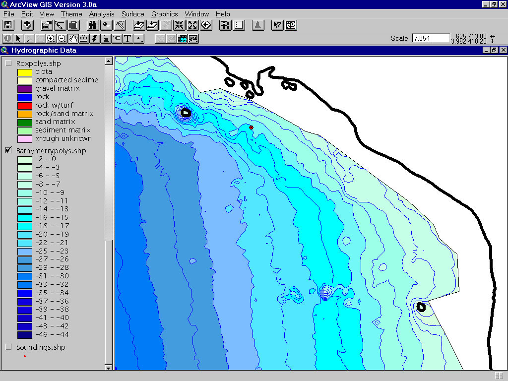
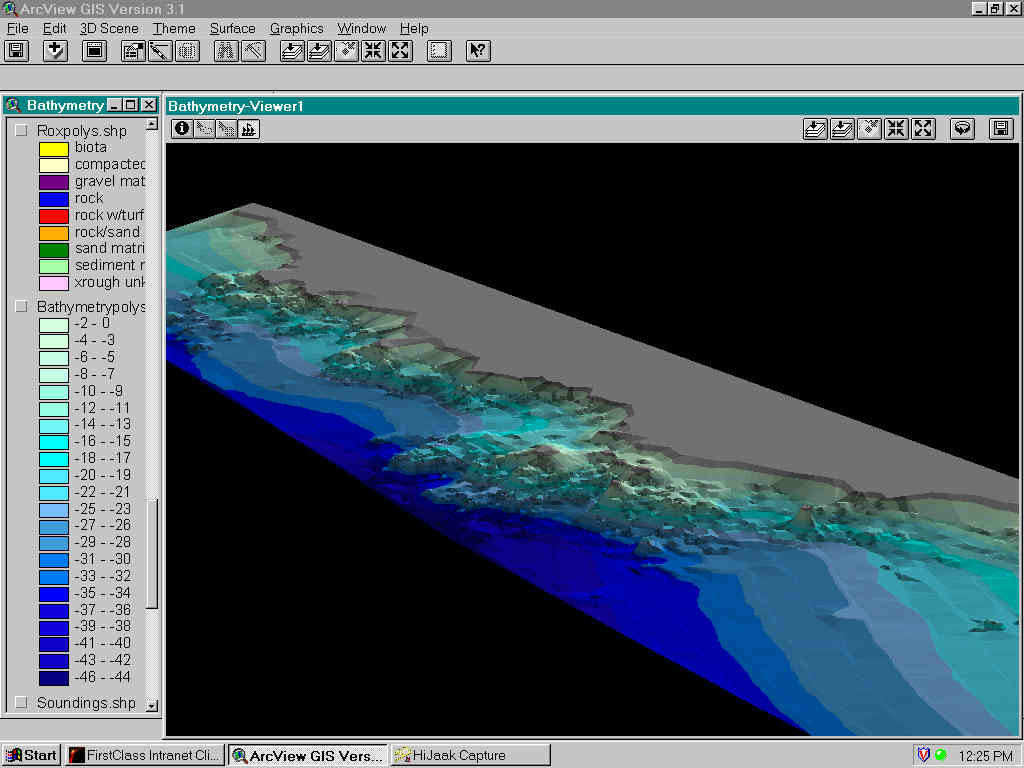
Figure 4.1 GIS products displayed in ArcView created for Big Creek Marine Ecological Reserve from x,y,z bathymetry data. Left) Two dimensional depth contour polygons can be used to stratify the site by water depth. Shoreline vectors (black lines) including offshore rocks can be used to define the "zero" depths when constructing the gridded bathymetry prior to contouring. Right) DEM of the same location shown in shaded relief and draped with depth polygons is used to illustrate slope, aspect, depth, and sea floor morphology simultaneously (Kvitek et al. unpublished data).
Figure 4.2. Illustration showing difference in coverage between singlebeam versus sidescan sonar and multibeam acoustic depth sounders (courtesy S. Blasco, Geologic Survey of Canada).
Information on substate type and texture can be collected as either point (x,y,z) data or as broad coverage raster imagery analogous to aerial photographs. Point data on substrate composition can come from georeferenced grab or core samples or even underwater photographs and video. Spatial resolution from this type of sampling, however, tends to be very limited due to the effort and cost required to increase data density while maintaining the spatial extents of the survey area. Point data on substrate type can also be acquired through co-processing or post-processing depth sounder data. For example, RoxAnn and Quester Tangent products make use of the multiple returns from echo sounders to classify seafloor substrates according to roughness and hardness parameters. This technology is similar to that applied in acoustic fishfinders, making use of the character and intensity as well as the timing of the return signal. With these add-on devices, it is possible to acquire information on the character of the substrate at each bathymetric sounding position. Similar approaches are now being developed for application to multibeam data. However, rigorous groundtruthing to verify that the resulting classifications are accurate is essential, because the results from this "automated" approach to seafloor substrate classification can vary widely between sites and with environmental conditions.
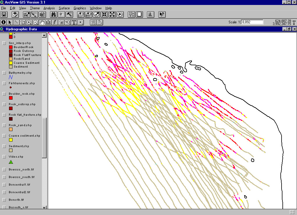
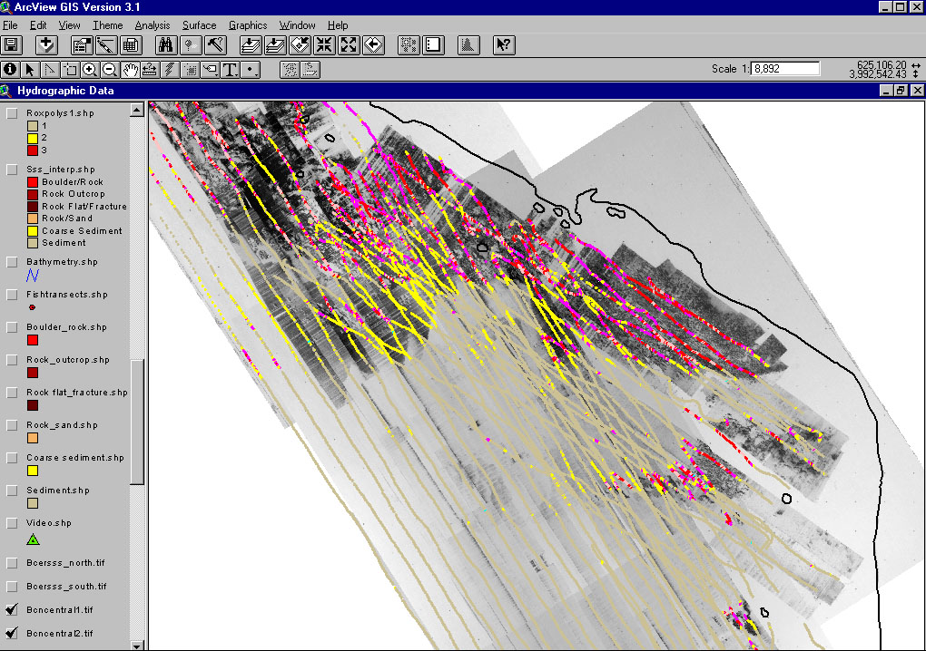
Figure 4.3 (Left) RoxAnn substrate classification data collected in conjunction with bathymetry data at the Big Creek Ecological Research. Red = rock, Yellow = cobble, Tan = sand. (Right) Same RoxAnn classifications varified against sidescan sonar imagery. (Kvitek et al. unpublished data).
Seafloor substrate raster data – acoustical methods
Seafloor substrate information can also be collected as continuous coverage raster imagery from reflected acoustic or optical backscatter intensity values. Because reflected intensities vary with substrate hardness, texture, slope and aspect, sidescan sonar has been used widely for over 30 years to create detailed mosaic images of seafloor habitats at resolutions as fine as 20 cm (Fig. 4.3). In recent years, this same approach has been applied to the backscatter values of multibeam bathymetry data (Fig. 4.4).
While multibeam backscatter images generally lack the resolutions and detail found in conventional sidescan images, they can be corrected for distortion resulting from unintended sensor motion (e.g. role, pitch, and heave due to waves). This type of correction has not yet been developed for sidescan sonar systems. As a result, shallow water sidescan sonar operations are generally restricted to days with relatively calm sea states, a rarity in may open coast areas. Multibeam systems equipped with motion sensors can be used under a much wider range of sea conditions. One other advantage multibeam systems have over sidescan sonar is continuous coverage directly below the sensor. Sidescan sonar systems have two side-facing transducers that do not ensonify the seafloor directly beneath the towfish.
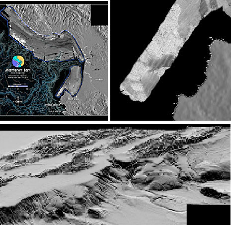
Figure 4.4 USGS high resolution bathymetry coverage in Monterey Bay, Ca. (a). Panel (b) shows multibeam bathymetry imagery from the inset. Panel (c) shows 3D digital terrain model fusion of offshore multibeam and terrestrial DEM data.
Seafloor substrate raster data – electro-optical methods
Optical techniques are also being developed for seafloor substrate mapping, including laser linescanner and multispectral imaging. Few of these instruments are in service at this time, in part due to their high cost and the still experimental nature of the technology. For this reason there is a scarcity of examples for comparison in terms of cost, quality, resolution, scale, etc. Nevertheless, these instruments show great promise; laser linescanners for their potential to dramatically increase image resolution over broad survey areas; and airborne multispectral systems for their ability to rapidly map habitat and vegetation types at meter resolution over vast areas in depths too shallow for survey vessel operations. As with all optical sensors, however, both of these technologies are limited in their depth range by water clarity. Below, we discuss the performance characteristics and costs associated with each of these new optical methods in greater detail.
Limitations to acoustic substrate acquisition techniques
Despite the high-resolution seafloor imagery obtainable using acoustic backscatter systems, their application can be limited by several factors including resolution, survey speed, swath width, and water depth.
The relatively slow survey speeds (4-10 knots) required for acoustic surveys can make mapping large areas at high resolution a long and costly enterprise. This situation is especially true in shallow water habitats due to the limitations imposed on swath width by water depth. For sidescan and multibeam systems, the closer the sensor is to the seafloor, the narrow the swath coverage. For most sidescan systems, swath width is limited to no more than 80% of the transducer altitude above the seafloor. Although multibeam systems can have very wide beam angles, data from the outer beams are usually of questionable value, especially in high relief areas where much of the seafloor at the edges of the swath is block from "view" due to acoustic shadowing by the relief. Survey track line spacing for shallow water surveys must therefore be closer than for deeper water work, where wider swath ranges can be successfully used. Even where wider swaths can be used, however, there is a trade off with resolution, which is directly and inversely proportional to swath width. (A sidescan sonar resolution of 20 cm at the 50 m range, drops to 40 cm at the 100 m range.)
Data acquisition in the very nearshore (0-10 m)
Although acoustic methods are not theoretically limited to a given depth range, several practical considerations generally preclude survey boat operations in the very nearshore (0-10 m). Wave height, submerged rocks, kelp canopy and irregular coastlines all make boat based survey operations difficult to impossible within this depth zone along the open coast. While a new technique has been developed for conducting acoustic surveys in kelp forests (see below), the other factors still argue for more efficient, safe and reliable means of mapping California’s extensive intertidal to shallow subtidal habitat. Airborne techniques including lasers and multispectral sensors, while limited to shallow water applications by their optical nature, may be the ideal tools for rapidly collecting elevation, depth, substrate and time series data along this vast and essentially unmapped zone.
4.2 CONSIDERATIONS IN SELECTING DATA ACQUISITION METHODS
A variety of remote and direct methods are available for acquiring depth and substrate data including: acoustic, electro-optical, physical and observational. Selection of which methods to use will be based on geographic extent of the project (scale) and the resolution required (data density), which in turn, are based on the purpose and goals of the project. Identifying the correct scale and resolution for a project in advance is important for two reasons. First, survey costs scale directly with each of these parameters, and there is generally a direct trade-off between scale and resolution if cost is to be held constant. As the aerial extent of a survey increases, resolution must decrease or survey time and costs will increase proportionally. Identifying the scale and resolution required for a given project is also an important consideration for selecting appropriate survey methods. If, for example, the goal is to simply map the aerial extent and depth of sandy versus rocky areas at mega- or meso-scales (1-10km) in moderate water depths (20-80m), then relatively low cost, low resolution techniques such as widely space acoustic survey lines would be adequate. Much higher resolution techniques would be required if the goal was to characterize the complexity of rocky reef habitats by quantifying the relative cover of specific substrate types (e.g. bolder fields, pinnacles, cobble beds, rocky outcrops, algal cover and sand channels), as well as sub-meter relief and the abundance of cracks and ledges because each of these meso- and macro-habitats supports a different species assemblage.
Once the scale, data resolution and budget for the project have been determined given the overall goal, it is then possible to move on to the selection of appropriate methods and tools.
In the following section we present a description of specific technologies commonly used or showing promise in the acquisition of depth and substrate data for nearshore benthic habitats. Wherever possible, we also present sample imagery and products as well as relationships between resolution, scale and cost.
The utility of bathymetric data is highly dependent on the resolution at which it is collected. Until recently most bathymetry data was collected as discrete point data along survey vessel track lines with singlebeam acoustic depth sounders. These sounders work on the principle that the distance between a vertically positioned transducer and the seabed can be calculated by halving the return time of an acoustic pulse emitted by the transducer. All that is required is an accurate value for the speed of sound through the intervening water column. The speed value can be back calculated by adjusting the sounder to display the correct depth while maintaining a known distance between the transducer and an acoustically reflective object (e.g. seafloor measured with a lead line, or calibration plate suspended at a known depth).
The horizontal resolution, or posting, of singlebeam acoustic data is defined by the sampling interval along the track lines and the spacing between track lines. Because it is generally impossible or too costly to space survey lines as close together as the interval between soundings along the track lines, most older bathymetry data sets tends to have much higher resolution along track than across track. This situation necessarily leads to considerable interpolation between track lines when constructing contours or gridded DEMs. As a result, the DEMs are generally either too course (postings at > 50m) or inaccurate for fine grain mapping at macro- or micro-habitat scales.
One advantage of single beam depth sounders however, is the ability to interface them with acoustic substrate classifiers. These co-processors correlate the intensity values from the single beam echo returns with seafloor substrate hardness and roughness.
Acoustic Substrate Classifiers
The most accurate method of bottom classification is that of in situ testing. Direct observations by SCUBA divers, drop or ROV video, or submersible provide substrate classifications with very high confidence levels, as do grab samples or cores; the latter two methods are especially useful for classifying sediments. However, application of these high-resolution, high-confidence methods of substrate classification in large area mapping projects can be quite costly in terms of money and effort. While class resolution of core and grab samples can be extremely high, the samples must be very closely spaced in order to give appreciable spatial (x,y) resolution. Similar obstacles exist for application of direct visual observation or video imagery to large areas; because of the limitations imposed by visibility underwater, cameras and/or observers must be placed in close proximity to the seabed that is to be classified, and achieving good bottom coverage becomes logistically difficult. In essence, drop camera samples are analogous to cores and grabs in that they are point samples, while ROV and submersible observations and video surveys may provide swath or area information within the visibility and physical range limits of their traveled course. Logistical constraints (in terms of cost, equipment required, support, etc.) can be quite high for ROV and especially submersible work. Towed camera systems may offer a considerably lower cost alternative to ROV or submersible observations while giving greater aerial coverage than drop cameras, but are also difficult to deploy in complex bathymetric settings, owing to the fact that they must be "flown" quite near the bottom due to visibility limitations. Over relatively flat bottom, or with very good visibility, however, these systems may be quite useful. All of these factors make direct observation of bottom type a much more appropriate tool for groundtruthing classifications derived from a remote sensing method with higher efficiency in covering large areas and lower cost per unit effort. Indeed, groundtruthing using the above methods is crucial when employing remote sensing techniques. In addition to providing greater coverage efficiency, bottom classifiers can help automate the classification process to some degree, especially relative to the human interpretation that must be applied to sidescan sonar or video imagery in order to map large areas. The primary means of remotely sensing and classifying substrate in the marine environment are acoustic methods.
The following text discussing acoustic substrate classifiers is drawn primarily from "Bottom Sediment Classification In Route Survey" (Mike Brissette, Ocean Mapping Group, Department of Geodesy and Geomatics Engineering, University of New Brunswick, http://www.omg.unb.ca/~mbriss/BSC_paper/BSC_paper.html#Bottom Sediment Classification). Additional text has been added, but the bulk of this section is quoted directly from that report.
This section will discuss two such sonars, namely Marine Micro System's 'RoxAnn', and Quester Tangent's 'QTC View'. Each discussion will look at the theory of operation behind each sonar as well as performance size requirements and costs.
ROXANN
Theory of Operation
RoxAnn is manufactured by Marine Micro Systems of Aberdeen Scotland. RoxAnn uses the first and second echo returns in order to perform bottom sediment classification. The first echo is reflected directly from the sea bed and the second is reflected twice off of the seabed and once off of the sea surface (Fig. 4.4). This method was first used by experienced fishers using regular echo sounders [Chivers et al, 1990]. The fishers observed that the length of the first echo was a good measure of hardness in calm weather.
Figure 4.4. Diagrammatic representation of first and second returns (from Chivers et al, 1990).
The second echo, which mimicked the first echo, was much less affected by rough weather. RoxAnn uses two values, E1 and E2, in order to estimate two key parameters of the sea floor, namely roughness and hardness. The first echo contains contributions from both sub-bottom reverberation and oblique surface backscatter from the seabed. It has been shown that oblique backscattering strength is dependent on the angle of incidence for different seabed materials. At 30 degrees there is almost a 10 dB difference in scattering level between mud, sand, gravel and rock [Chivers et al, 1990]. The first part of the first echo contains ambiguous sub-bottom reverberations and is therefore removed (Fig. 4.5). Most or all of the remaining portion of the first echo is then integrated to provide E1, the measure of roughness. The exact parameters within which E1 is integrated are difficult to estimate and is therefore based on empirical observations in a number of different oceans [Chivers et al,1990]. The entire second echo is integrated, which is the relative measure of hardness and is designated E2 [Schlagintweit, 1993]. A processor is used to interpret E1 and E2 such that bottom characteristics may be determined [Rougeau, 1989]. Looking at E1, on a perfectly flat sea floor, non incident rays would be expected to reflect away from the transducer. As the sea floor is not perfectly flat, the returning energy from non incident rays coincides and interferes with the incident rays and indicates the roughness of the sea floor [Chivers et al, 1993]. The specular reflection of the sea floor is a direct measurement of acoustic impedance relative to the sea water above it. Hardness can be estimated using E2 because the acoustic impedance is a product of the density and speed of longitudinal sound in the sea bed [Chivers et al, 1990].
Figure 4.5. First and Second Return Waveforms (from Schlagintweit, 1993)
Test Results
Schlagintweit [1993] conducted a field evaluation of RoxAnn in Saanich Inlet off of Vancouver Island using two frequencies, 40 kHz and 208 kHz. RoxAnn was deployed over a ground-truthed area that had been previously inspected by divers. A supervised classification method was used and a "modest" correlation was found at both frequencies. Classification differences between the two frequencies were due to the different sea bed penetration depths of these frequencies on various sea floor types. That is, the frequency dependent penetration factor into the sea floor depended on the local sea floor itself. Schlagintweit felt that the frequency should be chosen according to the application. Schlagintweit believed that an unsupervised classification method would be the best alternative, i.e., let the system select the natural groupings and then look at ground truthing. Both the Chivers et al [1990] and Rougeau [1989] articles support this method of an initial calibration. In separate tests, Kvitek et al [in press] found quite good agreement between classes created from sidescan sonar interpretation and those created using unsupervised classification of RoxAnn E1 & E2 values at the Big Creek Ecological Reserve in Big Sur, CA (Fig. 4.3). Using sidescan imagery and video groundtruthing, Kvitek et al found that RoxAnn successfully classified sand, rock, and coarse sand/gravel between 6-30m depth in a 2-3 sq. km area in this study.
RoxAnn Equipment
The RoxAnn system is very compact. The entire unit consists of a head amplifier (not shown) which is connected across an existing echosounder transducer in parallel with the existing echo sounder transmitter, and tuned to the transmitter frequency. The parallel receiver accepts the echo train from the head amplifier [Schlagintweit, 1993]. The installation requires no extra hull fittings, simply room for the processing equipment. The required processing equipment includes an IBM compatible computer and an EGA monitor [Rougeau, 1989]. Software which is specifically written to handle RoxAnn data must then be installed on the computer for processing analysis. The RoxAnn Seabed Classification System retails for about $15,000 US and the additional RoxAnn software costs about $10,000 US. Other programs such as Hypack, which retails for US$ 11,000, are also compatible with the RoxAnn hardware [Clarke, 1997]. These prices do not include taxes, installation expenses or services of a technician for calibration and sea trials.
QTC VIEW
Theory of Operation
QTC View is manufactured and distributed by Quester Tangent Corporation of Sidney, BC [Quester Tangent Corporation, 1997]. Like RoxAnn, Quester Tangent's QTC View uses the existing echo sounder transducer; however, QTC View does not examine two different waveforms. Instead, analysis is performed on the first return only. Quester Tangent's other classification system ISAH-S (Integrated System for Automated Hydrography) is also available, and uses the same approach as QTC View in wave form analysis. However, ISAH-S offers multiple channels for multi-transducer platforms, integration with positioning and motion sensors, and helmsman displays. QTC View is more of a standalone system accepting GPS input for georeferencing of echo sounder data. QTC View operates in the following manner. First, both the transmitted echo sounder signal and return signals are captured and digitized by QTC View. Second, the sea bed echo is located (bottom pick), and an averaged echo from several consecutive returns is computed [Prager 1995]. Next, the effects of the water column and beam spreading are removed such that the remaining wave form represents the seabed and the immediate subsurface [Collins et al, 1996]. Quester Tangent's echo shape analysis works on the principle that different sea beds result in unique wave forms. Through principal component analysis, complex echo shapes are reduced into common characteristics. Each wave form is processed by a series of algorithms which subdivides it into166 shape parameters [Collins et al, 1996]. A covariance matrix of dimension 166 x 166 is produced and the eigen vectors and eigen values are calculated. In general, three of the 166eigenvectors account for more than 95 per cent of the covariance found in all the wave forms. The 166 (full-feature) elements of the original eigen vector are reduced to three elements ("Q values"). These reduced feature elements will cluster around locations in reduced feature space corresponding to a sea bed type [Prager, 1995]. Test Results QTC View was designed to operate in both the supervised and unsupervised classification modes. If no ground-truthing has taken place in an area of interest, QTC View will still cluster-like areas such that some type of calibration or ground truthing may be performed after the survey. In a test conducted by the Esquimalt Defense Research Detachment, QTC View was found to have produced very good results. QTC View was used over the same area where the RoxAnn tests were conducted off of Vancouver Island in the unsupervised classification mode. QTC View was able to discriminate between eight different seabed types. After a calibration, QTC view was found to agree with each ground truthed area and showed good transition from seabed type to seabed type [Prager, 1995].
QTC View Equipment
QTC View is comprised of a head amplifier and PC with a DX2/66 processor. The head amplifier is connected in parallel across the existing transducer and to the PC via a RS232 cable. The PC also accepts the GPS data in NMEA-0183 standard GGA or GGL format for georeferencing of data [Collins et al, 1996]. The PC displays three windows: one for the reduced vector space, one for the track plot and classification and the third for seabed profile and classification. Figure 4.6 illustrates the QTC View screen output.
Figure 4.6. QTC View Screen Display (from Quester Tangent, 1997)
QTC is presently working with Reson, Inc. on adaptation of QTC View for use with multibeam depth sounders. This development will greatly increase survey efficiency by supplying substrate class data over most or all of the multibeam swath, but it is unknown when this product will be available. At present, however, QTC View will work with the Reson 8101 multibeam head, although it uses only the nadir beam data. QTC View retails for approximately US $15,000 [pers com J. Tamplin] [Lacroix, 1997] whereas ISAH-S retails for approximately $35,000 [Collins, 1997]. Unlike RoxAnn, the QTC View purchase price includes the software, and like RoxAnn the user must supply the computer. Hypack is not yet capable of acquiring raw QTC View data, but Coastal Oceanographics has provided support for recording the reduced dataset (3 "Q" values) processed in realtime by QTC view. The above prices do not include taxes or installation.
Summary
Both products discussed above have been shown to be useful tools for acoustic bottom substrate classification. The levels of success achieved in past studies using these tools is a function of the inherent qualities of the tools themselves, the operator and processor/analyzer expertise of those involved, the methods used, and the specific conditions of the areas studied. For this reason, true between-product comparisons are difficult. By far the most important fact to remember when using either of these tools (or any remote sensing method, for that matter) is that classifications created using these methods must be groundtruthed using one of the direct observation methods discussed above. Only with independent verification can confidence be placed in remotely sensed data.
During the last 10-15 years, use of multibeam bathymetry in hydrographic mapping has become increasingly common and accepted. Initially fraught with considerable accuracy and precision issues, multibeam sonar technology has improved vastly and rigorous testing has established its reliability. The ability to acquire denser sounding data while surveying fewer tracklines (with greater spacing between lines), and simultaneously acquiring backscatter imagery using the same sensor, has made multibeam a popular tool. Using this technology, however, requires attention to a number of considerations that are less crucial when using single-beam technology.
Multibeam depth sounders, as their name implies, acquire bathymetric soundings across a swath of seabed using a collection of acoustic beams (Fig. 4.7 left), as opposed to a single beam, which ensonifies only the area directly below the transducer. The number of beams and arc coverage of the transducer varies among makes and models, and determines the swath width across which a multibeam sounder acquires depth measurements in a given depth of water (Fig. 4.7 and 4.8). It is important to note that effective swath width is often somewhat less than potential swath width, as data from the outer most beams is often unusable due to large deviations induced by ship roll and interference from bottom features such as pinnacles. The potential swath width shown in Figure 4.8 may only be realized under calm conditions over a relatively flat bottom. Swath width is depth dependent, requiring closer line spacing in shallower water if full coverage is to be maintained. The mechanics and physics of how the beams are formed varies as well among makes and models, and may be a consideration of importance if extremely high resolution, precision, and accuracy are required.
Figure 4.7. (Left) Multibeam generated DEM of central California coast from shore to abyssal depths. Monterey Bay is at center right. (NOAA National Data Centers NDGC,
http://web.ngdc.noaa.gov/mgg/bathymetry/multibeam.html). (Right) Conceptual drawing of multibeam ensonification of seafloor (Kongsberg Simrad AS, http://www.kongsberg-simrad.com)In order for the multibeam system to calculate accurate x, y, and z positions for soundings from all off-nadir (non-vertical) beams (every beam other than the center beam), precise measurement of ship and transducer attitude is required. This includes measurement of pitch, roll, heading, and (preferably) vertical heave. Thus, a motion sensor must be interfaced to the unit, so that its output may be used to adjust and correct the multibeam data in either real time or post-processing.
Figure 4.8. Relationship between multibeam bathymetry transducer beam angle and swath coverage. For example: with a 90 degree beam angle swath width will be twice the water depth.
In addition, because of longer travel times for off-nadir beams, variations in the speed of sound in water (SOS) can induce relatively large errors in these beams; especially if temperature stratification exists in the water column. For this reason, sound velocity profiling should be conducted on site during a survey, and the SOS data used to adjust depth soundings. Controlling for variations in SOS is of increasing importance as depth increases. Multibeam surveying also requires more rigorous system calibration to account for systemic variations in, and improve the accuracy of, heading, roll, and pitch sensor values, as well as any adjustment to navigation time tags that will reduce timing errors between navigation and sonar data. This calibration, known as a "Patch Test", is typically conducted by running a series of survey lines over the same area with relative orientations that allow assessment of the variables listed above.
Multibeam bathymetric surveying generates orders of magnitude more data than single-beam surveying, resulting in greater storage requirements, longer processing times, and the need in some cases for greater processing power. Gigabytes of data may be generated daily, (as opposed to megabytes in single-beam surveys), especially if backscatter imagery is being recorded as well. The removal of bad sounding data during the editing process is, accordingly, a much larger task in multibeam than in single beam surveys, although some processing packages allow some degree of automation of this process.
The considerations and requirements listed above make multibeam surveying a much more complex and expensive undertaking relative to single beam, but the benefits in cost per unit effort and resolution can well outweigh the hardships, especially if extensive surveying is planned. Survey speeds of up to 30 knots are now possible with some systems. Minimal costs for setting up a multibeam system range from $75,000-$150,000 US for equipment alone, not including vessel, installation, and maintenance costs. Higher precision equipment with greater capabilities and more features can cost substantially more.
Sidescan sonar is the only technology capable of producing continuous coverage imagery of the seafloor surface at all depths. (Blondel and Murton [1997] give an excellent and comprehensive review of sidescan sonar theory, technology, imagery and application in their recent book, Handbook of Seafloor Sonar Imagery.) These systems transmit two acoustic beams, one to each side of the survey track line. Most sidescan systems use transducers mounted on a towfish pulled behind the survey boat (Fig. 4.2 & 4.9), but some are hull mounted. Because towfish can be deployed well below the water’s surface, they can be used in deeper habitats than hull mounted systems.
Sidescan sonar beams interact with the seafloor and most of their energy is reflected away from the transducer, but a small portion is scattered back to the sonar where it is amplified and recorded. The intensity of the backscatter signal is affected by the following factors in decreasing order of importance:

Figure 4.9. Klein sidescan sonar towfish about to be deployed from stern of survey vessel, and Klein 595 recorder printing hardcopy image (sonograph) of seafloor. Note black, port transducer running down the left side of the towfish (Klein Associates).
For each sonar pulse or ping, the received signal is recorded over a relatively long-time window, such that the backscatter returned from a broad swath of seafloor is stored sequentially. This cross-track scanning is used to create individual profiles of backscatter intensity that can be plotted along track to create a continuous image of the seafloor along the swath (Fig. 4.9).
Swath width is selectable but maximum usable range varies with frequency. High frequencies such as 500kHz to 1MHz give excellent resolutions but the acoustic energy only travels a short distance (< 100 m). Lower frequencies such as 50kHz or 100kHz give lower resolution but the distance that the energy travels is greatly improved (>300 m). Typical systems used for nearshore mapping have frequency ranges from 100 to 500 kHz with resolution as fine as 20 cm. Resolution also varies with swath width. Thus, while a 500 kHz system set at range of 75m will cover a 150m swath at 20 cm resolution, a 100 kHz system set at a range of 250m will cover a 500m swath but at a resolution closer to 1m. There is also a direct relationship between maximum allowable survey vessel speed and range. The shorter the range, the slower the speed and the more survey lines required to cover a given area. (Typical sidescan sonar survey speeds are around 4-5 knots, but with newer systems have been increase to 10 knots.) Thus, the trade-off between swath width, resolution, survey speed, and financial resources must be considered when planning a survey. The choices will depend on: 1) the size of the area to be surveyed, 2) what resolution of substrate definition is required, and 3) how much time and money is available for the survey. Interactive survey time estimate calculation tables such as the Hydrographic Survey Time Estimate Worksheet shown below can be easily constructed in a spreadsheet program such as Microsoft Excel. These tables can be used to construct what-if scenarios to explore the relative time requirements and costs for different survey parameters.
Another variable important to survey time is the amount of overlap desired between adjacent track lines. Most sidescan sonar systems cannot "see" the seafloor directly beneath the towfish. (Klein’s new multibeam sidescan system is an exception.) As a result, if complete coverage of the seafloor is required, it will be necessary to have up to 100% overlap of the sidescan swaths, such that the port side of swath along one track line is completely covered by the starboard side of the swath from the adjacent track line. In this manner, the outer range of one swath can be used to "fill-in" the missing inner-range of the adjacent swath during post-processing.
|
HYDROGRAPHIC SURVEY TIME ESTIMATE WORKSHEET |
||||||||
|
Client: CDF&G |
Project description: |
|||||||
|
Project Name: Big Creek Reserve Kelp Forest Survey |
Map & classify kelp forest/rockfish habitat |
|||||||
|
Preparation date: 18 April, 1996 |
Bathymetry, sidescan sonar, RoxAnn |
|||||||
|
Prepared by: Rikk Kvitek (831) 582-3529 |
||||||||
|
Survey area specifications |
Plan A |
Plan B |
Plan C |
Plan D |
||||
|
Survey area width (m) |
1,000 m |
10,000 m |
100,000 m |
100,000 m |
||||
|
Survey line length (m) |
1,000 m |
10,000 m |
100,000 m |
100,000 m |
||||
|
Line spacing (m) |
50 m |
50 m |
50 m |
500 m |
||||
|
Survey speed (knots) |
4 knots |
4 knots |
4 knots |
10 knots |
||||
|
Survey estimates |
||||||||
|
Number of lines |
20 |
200 |
2000 |
200 |
||||
|
Minutes per line (+1 for turn) |
9 min |
84 min |
834 min |
334 min |
||||
|
Total survey time (hours) |
3 hr |
281 hr |
27811 hr |
1114 hr |
||||
An additional advantage of designing overlap into the survey is to provide different views of the seafloor. This approach is especially important in areas of high relief, where features such as rock pinnacles may block the acoustic beam from striking and reflecting off that part of the seafloor hidden from towfish view. This interruption of the acoustic beam will create shadows or blind spots in the record, which can be filled with information from adjacent tracklines if there is sufficient overlap. Running track lines at different angles over the survey area can also be used to give a more complete picture of what the habitat looks like. For example, the acoustic appearance of canyons, pinnacles and exposed rock strata can vary greatly with approach angle.
Once the survey is completed, the swath images or sonographs can then be combined into a composite image or mosaic of the entire area surveyed (Fig. 4.10). Traditionally, these sonographs were created as hardcopy originals by the sidescan recorder, but are now more often recorded in digital form. As a result, all post-processing, including image enhancement, mosaicking and GIS product creation can be done electronically. Interfacing the sidescan with a differential GPS navigation system can produce georeferencing and imaging accuracy at submeter resolutions. To obtain this accuracy, however, requires that the off-set or "layback" between the sidescan sonar transducer and the GPS antenna is accurately determined and recorded throughout the survey.
Figure 4.10. Sidescan sonar mosaic of Big Creek Ecological Reserve, Big Sur, California produced with an EG&G 260 100 kHz towfish sidescan sonar system (authors’ unpublished data).
The sonographs and mosaics are used to create what is know as a sidescan interpretation. This process involves tracing polygons around regions of similar substrate as identified on the sonograph (Fig. 4.11). While it is relatively easy to differentiate between rock and sediment on the sonograph, caution must be exercised in the interpretation of the substrate based solely on the sidescan imagery if finer division of the substrate type is required (e.g. cobble, gravel, coarse sand, fine sand, silt, clay, etc.). As a result, it is often necessary to augment the sidescan data with some form of direct sampling (scuba, video, ROV, bottom grabs, etc.) in order to groundtruth the interpretation.
Groundtruthing is especially critical when image analysis software first developed and refined for use with satellite imagery is used to automate the classification and interpretation of the sidescan imagery. Classification involves identifying different features or classes in an image based on their reflectance characteristics. There are two principal methods for performing a classification of an image. "Unsupervised classification" is a method for grouping pixels in an image into classes or "clusters", based on their statistical properties, without the user supplying any prior information on the classes. Once the unsupervised classification has been performed, the clusters that the classifier has identified can be examined and labeled according to what class they represent in the real-world as determined via groundtruthing.
"Supervised classification" involves the user first "training" the system in recognizing different classes by selecting representative samples of each class or habitat type from the image: these samples are known as training sets and should be groundtruthed prior to performing the supervised classification. The system then assigns each pixel in the image to one of these pre-determined classes. Some groundtruthing is essential for accurate classification results regardless of the method used. While highly effective in processing aerial imagery of terrestrial habitats, development of classification techniques is still in its infancy for application to acoustically derived images of marine habitats. These classification routines are available in stand-alone image processing software packages such as ERDAS and DIMPLE, as well as accessories or modules for some GIS software packages including those offered by ESRI and MicroImages.
Once processed and correctly georeferenced, the sidescan imagery and interpretations can also be draped over DEM’s to give a 3D representation of the seafloor (Fig. 4.12).
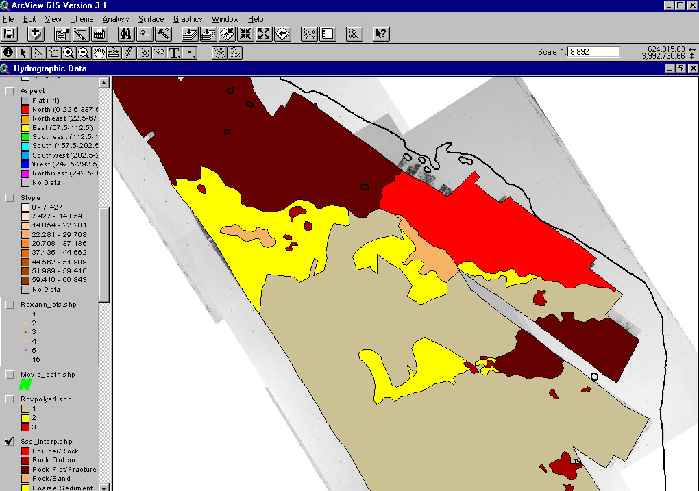
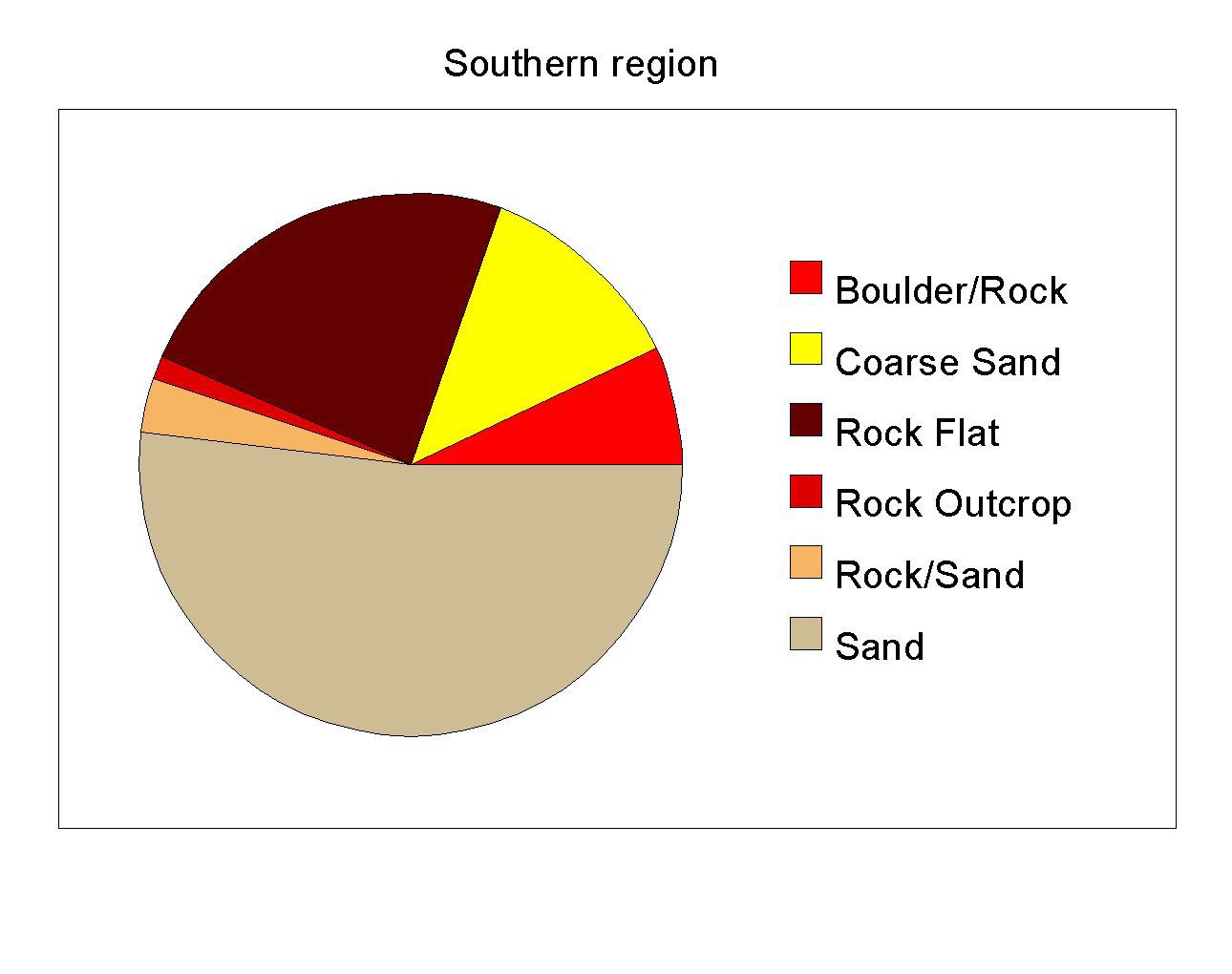
Figure 4.11. Sidescan sonar interpretation created from mosaic shown in Figure 4.10 of the Big Creek Ecological Reserve, (authors’ unpublished data).
Figure 4.12. Sidescan sonar mosaic draped over DEM of Big Creek Ecological Reserve, (authors’ unpublished data).
SPECIAL CHALLENGES TO SIDESCAN SONAR SURVEYS IN SHALLOW WATER
Challenges specific to shallow water nearshore marine habitats make sidescan sonar surveys in these areas more difficult, and costly than for deep water offshore surveys. Close to shore, waves are often higher and small vessels must be used where larger ones will serve in deeper waters. These factors combined with the shorter cable lengths required for shallow water surveys mean that under a given set of conditions, there will be more wave induced vessel motion transferred to the towfish during a shallow water versus a deep water survey. Any towfish motion other than along track movement (e.g. pitch, yaw and heave) will create distortion in the sonograph. While motion sensors are available for single beam and multibeam bathymetry systems, they have not yet been developed to remove motion induced distortion from sidescan sonar data. For this reason, shallow water sidescan sonar surveys conducted when seas are > 2m produce results of little value.
Geohazards
Geohazards are also more of a consideration in shallow waters because towfish altitude above the seafloor is often limited by water depth. Towfish altitude should be kept between 10% and 40% of the range if full coverage of the selected swath width is desired. Less than 10% will result in loss of signal from the outside part of the range, and greater than 40% will produce a large gap in coverage directly below the fish. In water depths of > 40m a towfish could be kept up to 40m off the bottom while still maintaining a range of 100m on a side. This margin of safety is not available, however, in water depths of 10 to 30 m, where the towfish must be kept at least 10m off the bottom but cannot be raised more that the water depth. Thus, a 20m pinnacle in 30m of water presents a very serious hazard to sidescan operations. For this reason, it is always advisable to conduct a bathymetric survey prior to the sidescan work in areas of uncertain seafloor morphology.
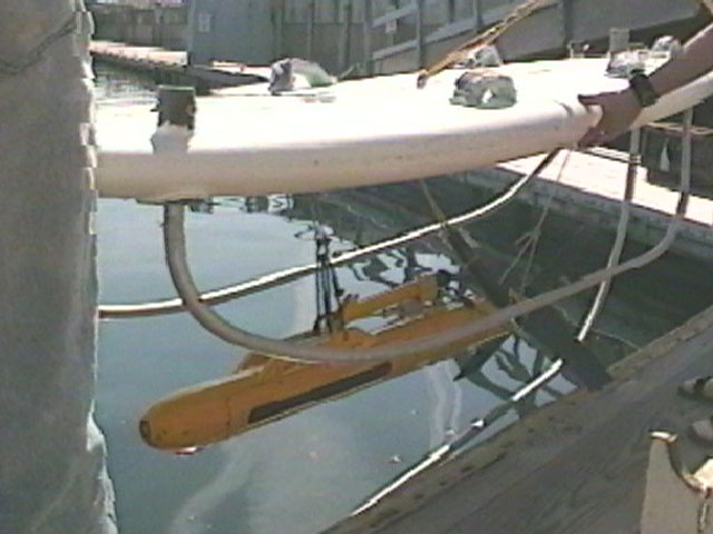
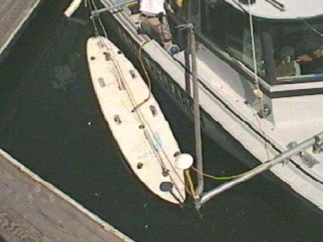
Figure 4.13. (Left) Sidescan towfish suspended from towed surface float (surf board) and protected by three kelp deflection bars. (Below) "Kelp board" deployed in survey mode with sidemount on survey vessel. Note GPS antenna on outboard end of sidemount arm.
Kelp
Kelp canopy presents another hazard for shallow water sidescan work. Although a survey vessel may be able to motor through a sparse kelp canopy, even the smallest amount of kelp that snags on the towfish will result in distortion of the sidescan record due to erratic motion of the towfish. The seafloor mapping group at California State University Monterey Bay has developed a system for shielding their towfish from kelp as it is towed through canopy cover, and are now routinely surveying in area previously off limits to sidescan (Fig. 4.13).
In summary, the advantages of sidescan sonar for habitat mapping are that these systems can produce continuous coverage georeferenced digital imagery of the seafloor substrate at resolutions on the order of decimeters. This technology is analogous to the use of aerial photography for mapping habitats in terrestrial systems. The constraints imposed by the aquatic medium, however, make sidescan sonar a costly endeavor. Vessels are slower than aircraft, sidescan systems are more expensive than cameras, sound energy attenuates more rapidly in water than light does in air, and airplanes need not fly through tree canopies to get their imagery. Costs for complete sidescan sonar systems including dGPS navigation interface and digital data acquisition and processing start at over $150,000.
4.4 ELECTRO-OPTICAL MAPPING TECHNIQUES
In recent years, several new technologies have emerged that may be applied to coastal marine habitat mapping; these tools rely upon the electro-optical, rather than the acoustic, spectra to make measurements and create imagery. Three main types of electro-optical tools show great potential for use in habitat mapping: CASI, LIDAR, and laser line scan (LLS). Two of these tools (CASI and LIDAR) are aircraft-deployed, offering great improvements in vessel speed and survey efficiency (but with lower resolutions in some cases), while the third (LLS) is typically deployed in a towed body similar to sidescan sonar systems. Each tool has specific capabilities, limitations, and considerations, which will be addressed in detail below.
Compact Airborne Spectrographic Imager (CASI)
The Compact Airborne Spectrographic Imager (CASI) system, developed by ITRES Research Ltd., is a imaging system with a two-dimensional CCD array and reflection grating to provide spectral dispersion of the incoming optical signal. The CASI instrument is described in detail in the account of its use in the BOREAS project (Earth Observations Laboratory, http://www.eol.ists.ca/projects/boreas/) and consists of five modules: Sensor head, Instrument Control Unit, Keyboard, PowerSupply Module and Monitor (Fig. 4.14).
Figure 4.14 CASI-2 system manufactured by Itres Research, Ltd.
The following text is directly paraphrased from that document. Total instrument weight is 55 kg. Power requirements are 110 volts at 2.4 amps and with a suitable inverter the CASI can be operated from the 28 volts DC power found on many aircraft. Designed to be compact enough to be flown on light aircraft, the CASI has been flown on quite small aircraft such as the Piper Aztec and Cessna Citation. With no moving parts to the optics, the CASI is a "push broom" imaging spectrograph with a reflection grating and a two-dimensional CCD (charge coupled device) solid-state array detector.
The CCD sensor is a P86520 series frame transfer device (EEV Inc. Chelmsford, UK). The array is thermoelectrically cooled to 2 C to reduce dark current. The imaging area of the array is 578 x 288 pixels with each element measuring 15.5 by 22 um. The instrument operates by looking down and imaging a line perpendicular to the aircraft line of flight. A two-dimensional image is created as the forward motion of the aircraft allows the imaging of successive lines under the aircraft (Anger et al. 1990). The reflection grating provides spectral dispersion of the incoming optical signal. CASI has a nominal spectral range of 391 nm to 904 nm with a spatial resolution of 512 pixels across the 35-degree field of view (FOV). Ground resolution depends on the aircraft altitude and ranges from one to ten meters. The spectral resolution is nominally 2.5 nm FWHM (full width, half-maximum), with 288 spectral channels centered at 1.8 nm intervals. This bandwidth increases with wavelength. The CCD sensor is read and digitized to 12 bits by a programmable electronics system, which is controlled by an internal single-board computer. Data are recorded on a built-in digital tape recorder (Exabyte) which uses 8 mm cassettes, or to other removable or hard disk media. This low cost, standardized, data storage medium greatly facilitates post processing of the data. Each tape can store up to one gigabytes of data or depending on the frame-rate up to one hour of imagery. A representative value for the frame rate under typical conditions is 20 frames (lines) /sec for eight spectral channels in imaging mode. Due to the high data rate of the CASI sensor, three user selectable operating modes have been developed. Each mode maximizes the information content while keeping the data rate at a manageable level.
Figure 4.15 Diagram of CASI in Imaging Mode (IM), showing spatial and pixel coverage (Earth Observations Laboratory, http: //www.eol.ists.ca/projects/boreas/)
The three operating modes are Imaging mode (IM), multispectral mode (MS), and Full-frame mode (FFM). In IM, full spatial resolution of 512 spatial pixels across the 35 degree swath is achieved (Fig. 4.15).
Channel wavelengths and bandwidths are user specified (up to 15 bands). In imaging mode, the image width is 512 pixels, and the image length is determined by the length of time that the imager is allowed to operate. Each picture element records radiance values in up to 15 bands between 391 and 904 nm, the spectral location of the bands being selectable by the operator. The pixel size is approximately 1 m by 2 m, when the aircraft is flown at 2000 m above the target surface. Slowing the aircraft substantially may be able to reduce pixel size to as little as 60 cm, but to accomplish this one must reduce the number of bands to about 10 or use band averaging to 16 nm wide bands. Imaging mode is also sometimes called spatial mode.
In multispectrometer mode (MSM, Figure 4.16), full spectral resolution of 288 channels for up to 39 look directions across the 35 degree swath are possible. Look direction spacing and location are user specified to sample the array. This sampling produces an image rake or comb.
A single channel, full spatial scene recovery channel can be selected. In multi-spectrometer mode, the image width is up to 39 pixels, the image length is determined by the length of time that the imager is allowed to operate, and each picture element records the radiance values at up to 288 wavelength intervals in the region from 391 nm to 904 nm. The pixel width is the same as that in imaging mode, however adjacent pixels on the image represent ground points separated by approximately 20 m. The pixel length is approximately 6 to 8 m, and depends on the speed of the aircraft, and on the integration time selected. When the imager is operated in multispectrometer mode, it produces a second image, called the "track recovery row", which consists of only one spectral interval, but is at the spatial resolution of the imager when operated in spatial mode. This track recovery image is usually used solely for locating the multispectrometer image, although it could be included as part of the data stream. This mode is also sometimes called spectral mode.
Figure 4.16. Diagram of CASI in Multispectrometer Mode (MSM), showing spatial and pixel coverage (Earth Observations Laboratory, http:// www.eol.ists.ca/projects/ boreas).
In full-frame mode (FFM, sometimes called calibration mode, CASI outputs all the 288 spectral channels for all 512 spatial pixels (i.e. the whole array). This mode requires long data readout times, in the order of one second or more. In airborne operation the first two modes are typically used in successive flights of the same target area. The full-frame mode is used for calibration and ground measurements. CASI has been used successfully in terrestrial, freshwater, and marine settings, to map vegetation, substrate, phytoplankton abundance, thermal and pollution plumes, and other features. By imaging reflectance in different spectral brands, vegetation can be distinguished taxonomically, to species in some cases. In the marine environment, CASI has been used to map benthic algae and substrate type in one of the largest airborne mapping projects to date, to map benthic habitats in shallow coastal waters in Port Phillip Bay, Australia (Anstee et al., 1997, Figs. 4.17 and 4.18).
Figure 4.17 Benthic cover classification using CASI (Anstee et al., 1997, http://www.clw.csiro.au/research/environment/remote/australia.html).
This large embayment adjacent to Melbourne has an area of about 1,950 km2. It is relatively shallow with over half the area being less than 10 m deep. Urban population and industrial development on its shores has been increasing, creating growing pressures on the bay’s ecology and water quality.
Figure 4.18 Color image mosaic created using CASI (Anstee et al., 1997, http://www.clw.csiro.au/research/environment/remote/australia.html).
The CASI was used to map the whole of the bay to a depth of 15 m (the major portion of the bay), to derive maps of benthic type and cover to 1:25,000 map accuracy, and to help develop objective ecological categories to provide a base for monitoring. Starting with 6 GB of raw CASI data (72 flightlines) at 5 m pixel resolution, laboratory and field methods were developed for mapping spectrally distinguishable benthic materials and optical water quality in the bay. The major breakthroughs of this work, conducted by CSIRO, included the ability to treat the data as physical reflectance, to use large mosaics on a consistent physical basis as ‘single’ images, and (through physical modeling) to abolish the need for coincident in-water data collection.
An important consideration when using CASI, as with other electro-optical methods, is water clarity. Turbid or otherwise poor-visibility conditions reduce the depth capabilities and resolving power of CASI. A rule of thumb is that CASI is generally effective only within approximately the secchi depth, typically 5-15 m in coastal California waters < 30m deep. Positional accuracy of CASI data is dependent upon type of GPS positioning used (i.e. differential or RTK GPS) and accuracy of aircraft attitude sensor used (as with all airborne data collection methods, aircraft pitch, roll and yaw must be accounted for). Accuracies of ± 2m are common with dGPS. CASI may be deployed simultaneously with LIDAR, achieving greater survey efficiency by simultaneously collecting two types of complementary data (see below).
LIght Detection And Ranging (LIDAR) technology has been used to map topography and bathymetry, and to detect objects (mines, fish schools, etc.) in the water column in marine and freshwater bodies of water. As with CASI, LIDAR is deployed from an aircraft, either fixed-wing or helicopter. Systems for hydrographic mapping typically use a blue-green laser (532 nm) to optimize penetration depth. One such system, the SHOALS (Scanning Hydrographic Operational Airborne LIDAR Survey system) (Fig. 4.19), operated by USACE, is capable of mapping both coastal topography and nearshore bathymetry simultaneously, by the addition of a dual-frequency IR laser.
Figure 4.19 SHOALS LIDAR system (http://shoals.sam.usace.army.mil/).
One half of the altitude-dependent swath-width must be over water for this to function; at normal altitude (200m), this allows a 50 m portion of the terrestrial coastline to be mapped. Other LIDAR systems optimized for terrestrial mapping might then be used if terrestrial elevation data beyond this 50 m swath are desired. Under normal operating conditions (an altitude of 200 meters and a speed of 60 or 120 knots) the system can survey up to 8-32 square kilometers in one hour, collecting depth soundings on a 4 meter horizontal grid. Using dGPS, SHOALS references each depth measurement to a horizontal position accurate to 3 meters and a vertical position accurate to 15 centimeters. RTK GPS can increase the horizontal accuracy to the sub-meter level. Water clarity affects the depth capabilities of LIDAR; under ideal conditions, up to 60 m penetration is possible. In a project in Redondo Beach, CA, 20-25 m penetration was achieved.
Georeferenced video is recorded simultaneously with the SHOALS LIDAR depth & elevation data. This imagery may be used to help interpret data inconsistencies and to construct mosaics of aerial imagery. As mentioned above, LIDAR may be co-deployed with CASI. Use of the SHOALS system costs $8,000-$10,000 US per square mile (approximately $3100-$3900 per square km), depending on whether dGPS or RTK GPS is used. For this price, both raw and processed x, y, z data are provided on a CD-ROM, as well as raw video imagery if desired (CASI is not included and must be arranged separately).
Unlike the previous two tools, laser line scan (LLS) systems are deployed either in towed bodies similar to a sidescan sonar fish, or on submersibles. This tool, originally developed by the military for mine hunting applications, uses laser light to create high-resolution seafloor imagery (Fig. 4.18). LLS systems were used recently in the search for the TWA 800 and Swissair 111 air disaster remains. A solid state blue-green laser is continuously scanned across a 70º field of view illuminating only a pencil diameter spot at any one time. This spot is tracked by a highly sensitive narrow beam sensor, thereby vastly reducing the effects of backscatter from waterborne particles. The data from the receiver are digitized in real time and stored in an image buffer for display, line by line, on a conventional video monitor, and stored on computer disk for further processing. Data volumes generated are dependent upon resolution, but are substantial (GBs). Potential resolution is much better than that provided by sidescan sonar, as fine as 1 mm. LLS thus provides a resolution midway between that provided by video and still imagery, but at a much higher coverage rate and with much better penetrating capabilities (up to four or five times that of video, Table 4.1). As with video, water clarity limits viewing altitude, and thus swath width and resolution possible (Tables 4.2, 4.3). Survey speeds of 1 to 6 knots are possible, in water from 3 to 1500 m deep. At present, systems manufactured by Northrop-Grumman (formerly Westinghouse) and Raytheon Corporation are available, although high purchase price and related costs may make contracting survey companies offering LLS services (such as SAIC) a more viable option. Additionally a single multi-spectral LLS system exists, owned and operated by the U.S. Navy. At present, it can be deployed only on a submersible. This system and its uses are described in Strand et al., 199X, (
http://www.ncsc.navy.mil/css/papers/oceanopeoid.htm). The fundamental difference between this sensor and more conventional laser line scan systems, such as the CSS/Raytheon EOID Sensor or the Raytheon LS-4096, is the fact that this sensor has four separate receivers (Fig. 4.20).
Figure 4.20. Multi-spectral LLS system owned by U.S. Navy and used in the CoBOP Program (Strand et al., 199X).
Each receiver consists of a rotating optical assembly, a controllable aperture assembly, a photo-multiplier tube (PMT), a preamplifier and signal conditioning electronics, and an analog-to-digital converter (ADC). Each of the receivers’ rotating optical assemblies can be fitted with optical interference filters and other optical elements, such as polarization analyzers, which allow various aspects of the reflected light field to be evaluated. In a conventional laser line scan system, the receiver is used to measure the magnitude of the reflected light field and the receiver is therefore fitted with no filter or with a filter whose center wavelength matches the wavelength of the outgoing laser light. The use of an optical filter in this case helps reduce the undesirable energy due to ambient sunlight or auxiliary luminaries that may be mounted on the deployment platform. During the CoBOP Program (Strand et al., 199X, http://www.ncsc.navy.mil/css/ papers/oceanopeoid.htm) the multi-receiver laser line scan system was used to investigate biological fluorescence by using a short wavelength laser and fitting the receivers with optical filters whose center wavelengths correspond to known fluorescence wavelengths. An Argon Ion laser whose output was tuned to 488nm was used as the stimulating light source and three of the receivers were fitted with interference filters. A 680nm (20nm FWHM) filter was installed in channel #1, a 570nm (40nm FWHM) filter was installed in channel #3, a 515 nm (20nm FWHM) filter was installed in channel #4, and channel #2 was left open without any filter. When the system is used to create color images the Argon Ion laser is replaced with an Argon/Krypton mixed gas laser which provides simultaneous outputs at 647nm (red), 515nm (green), and 488nm (blue). Matching filters, with 6nm FWHM bandwidths, are then added to three of the four receivers and the data required to produce RGB color images can be collected. The images presented in Strand et al. (199X) demonstrate that the quantity and quality of target related information produced by a laser line scan system can be increased dramatically by evaluating other linear and non-linear, or elastic and inelastic, characteristics of the light field.
Table 4.1. Comparison of potential range (or viewing altitude, expressed in terms of R, the range of video camera & light systems), resolution, and search rate for camera and laser line scan systems. Source: SAIC.
Colorful RGB images, for example, can be produced by illuminating the object with a multi-colored laser and simultaneously monitoring the magnitude of the reflected light at three coordinated wavelengths (Figs. 4.21-4.24). The color images produced in this manner have been shown to be very realistic and could be produced at a range that was 8-10 times greater that the range at which a three chip color CCD television camera was able to produce useful color information. These images also demonstrate conclusively that inelastic, or trans-spectral, phenomena such as fluorescence can also be used to great benefit. Fluorescence maps can be produced that describe, on a point-by-point basis, the fluorescent characteristics of large and small individuals within a relatively large, panoramic field of view. While the importance and application of these fluorescence maps is just beginning to be explored, the intimate connection of fluorescence with key biological processes makes the potential utility of FILLS imagery appear to be particularly tantalizing. Possible applications of these new image forms include wide area evaluation and assessment of specie diversity and distribution, the study of inter-relationships between species and individuals, evaluation and mapping of the health and biological vigor of coral reef communities, and the possible localization and identification of pollutants and other negative stress factors.
Table 4.2. Comparison of resolution, positional accuracy, coverage rate, and sea bottom impacts for sidescan sonar, camera, and laser line scan systems. Source: SAIC.
Table 43. Effect of water clarity on potential imaging altitude, swath width, coverage rate, and resolution for laser line scan systems. Source: SAIC.
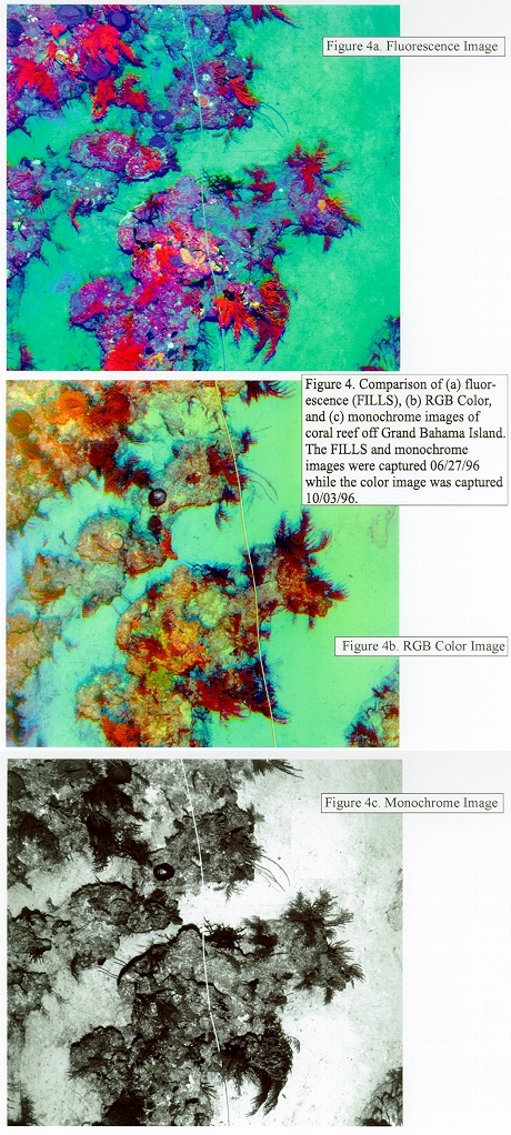
Figure 4.21. Comparison of LLS Fluorescence, RGB Color and Monochrome Images. (Source Strand et al, 199x).
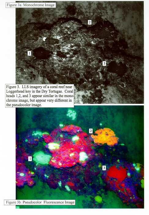
Figure 4.22. Comparison of LLS Monochrome and Pseudocolor Fluorescence Images. (Source Strand et al, 199x).
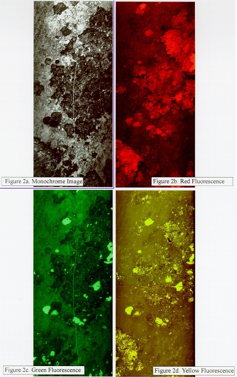
Figure 4.23. Comparison of Monochrome LLS Image, Red Fluorescence, Green Fluorescence, Yellow Fluorescence. (Source Strand et al, 199x).
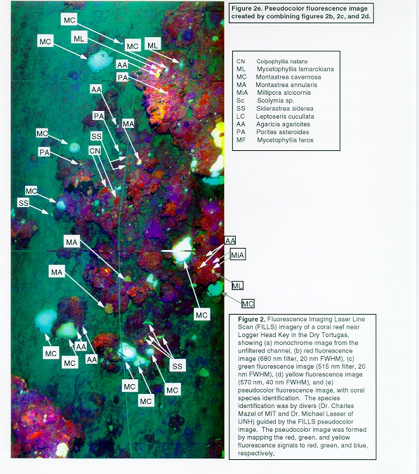
Figure 4.24. Pseudocolor LLS Image created by combining Red Fluorescence, Green Fluorescence, Yellow Fluorescence (source Strand et al, 199x).
4.5 DIRECT 1:1 SAMPLING METHODS
Despite the remarkably fine resolution now achievable using acoustic and electromagnetic remote sensing techniques, direct or 1:1 sampling (scuba observation, cores, video, etc.) is still critical to the success of any subtidal mapping program for at least three reasons. First, while remote sensing technologies are capable of submeter resolution, much of the habitat detail important to the biotic communities can occur on the scale of centimeters. Grain size, small cracks, pits and mounds that may be below the resolving capabilities of remote sensing systems can be sampled using direct techniques. Secondly, some types of biotically important features, such as void spaces between rocks, can be difficult or impossible to accurately quantify in terms of size and distribution using acoustic techniques. Finally, if accurate habitat maps are to be produced from remotely sensed data, the results need to be groundtruthed using direct methods. For example, a white area on a sidescan sonograph is the result of no or very low reflected signal. Without directly sampling the area, the operator may not be able to determine whether the light patch is a region of very soft sediment which reflected little of the signal, or a shadow cast behind an object projecting up into the water column. Although this is an extreme case, the issue remains that sonographs are merely spatial patterns of acoustic reflectance which often have to be "spot-checked" with direct techniques if the true nature of the substrate is to be identified (e.g. grain size, rock type, biotic cover, etc.).
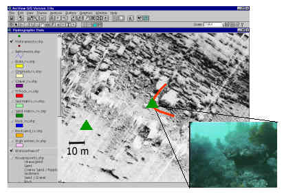
Figure 4.25. Multimedia GIS. Symbols can be selected to display georeferenced digital still images (green triangle) or video movie clips from a underwater video transect (red path) embedded in a GIS theme displayed over a sidescan sonograph
.Underwater positioning and georeferencing
A variety of methods are available for groundtruthing and 1:1 sampling of the seafloor including: direct observations by scuba divers, diver operated still and video cameras, sediment cores and grabs, drop cameras deployed from a vessel, submersibles, and remotely operated vehicles (ROV) guided by a pilot from a deployment vessel. Common to all of these methods, however, is the need for accurate georeferencing of where the samples are collected. Again, there are a variety of methods for determining the x, y, z location of were a sample is taken. The simplest methods for geolocating sampling locations involve determining the surface position of the deployment vessel using GPS and assuming the location of the sample is directly below the boat or float. This approach is most successful for cores, grabs, and drop-cameras used in areas of low current and wind, such that the cable or tether remains nearly vertical.
Under circumstances where there may be significant horizontal displacement of the sampling device away from the deployment vessel, such as with divers and ROV’s, some type of underwater tracking will be required if meter level resolution is required. Acoustic tracking systems, such as DiveTracker from Desert Star and Track Point II
® from ORE International, can be used for underwater tracking and navigation in real-world coordinates when interfaced with dGPS. Using these systems, divers, submersibles, and ROVs equipped with video cameras can be precisely guided along pre-determined transect lines. These georeferenced video images can be incorporated directly into GIS products as snap shots or "move clips" to illustrate what the habitat actually looks like (Fig. 4.25) (Bretz, Kvitek and Iampietro 1998). Also, when equipped with paired reference lasers set a known distance apart, video transects and quadrats can be used to quantify the size, distribution and abundance of many habitat features as well as species. Vertical images of the seafloor, if precisely georeferenced, can even be mosaicked to produce continuous, highly detailed views of larger areas (Fig. 4.26). Furthermore, with the advent of digital video imagery, these mosaic images can be greatly enhanced to reveal much detail normally obscure in conventional analogue imagery (Howland et al. 1999).
Figure 4.26. Example of georeferenced seafloor video mosaic. Image is of hypoxic brine pool found at 10m water depth in Resolute Bay, Canada. Picture was created from four digital video stills images (Kvitek et al. 1998).
5. DATA ACQUISITION TOOLS AND PROVIDERS DATABASE
Part of Task 3, as defined in the California Department of Fish and Game (DFG) Nearshore Ecosystem Database Project (NEDP) was to collect information on remote sensing technologies applicable to nearshore habitat mapping. This information was to include:
Here we define "tool" as any piece of hardware or software that is used for acquisition, processing or display of bathymetric or backscatter data. Our goal was to create a database containing this information in a format useful to DFG personnel charged with planning, acquiring or using benthic habitat mapping data from nearshore, shallow water environments. Our objective was to collect, organize and present all relevant information in a useable database. The following categories were used to organize the information: Tools, Tool Manufacturers, Survey Service Providers, Survey Equipment Providers, University Contact List, University Capabilities, and Government and Non-Profit Agencies. Our general approach was to first identify the types of tools most commonly used for acquiring seafloor depth and substrate data as well as new technologies that show promise for shallow water mapping. Once the list was developed, the next objective was to contact as many reliable sources possible to gather information about the relative performance and costs of using these tools, as well as service providers available on the West coast. This information was then compiled into the table presented below as well as a Microsoft Access database as requested by DFG.
A list of common tools was obtained from published reports, personal contacts, trade journals conversations, information packets and survey service provider websites.
Prior to beginning our search for information, a database was developed in Microsoft Access for archiving the information and to allow for queries and relational searches. Data tables were created for each type of entry (tools specification, provider services and costs, etc.), and where appropriate tables have been linked to another table via an intermediate relational table. A unique ID number has been assigned to each entry, and these ID numbers have been placed in a relationship table to allow for crossover queries. Forms have already been developed to aid in, and display the results from the most common types of queries likely to be performed by DFG. Although there is more information in the database than reflected on the current forms, these forms can be easily adjusted to fit specific needs. New relationships and forms can also be created as needed.
While the database was being setup, a preliminary search for information was done using the web, industry and scientific journals (i.e. Sea Technology, Geology, etc.), and personal contacts. This search was used to create lists of those manufactures, service providers, universities, survey equipment providers, and agencies capable of meeting DFG mapping needs. Our focus was on technologies suitable for the acquisition and processing of seafloor depth and substrate data along the California continental shelf, with special attention given to the shallow nearshore (0-30 m depth).
Manufacturers were first asked to fax information packets to aid in our initial evaluation of tools. Tools specifications and prices were recorded. Manufactures were then re-contacted to obtain references for relevant tools and any information unavailable in the information packets. Tools were then tabulated and placed in categories such as: multibeam, side scan sonar, processing and acquisition, seabed classification systems and electro-optical systems. Common questions asked were based on model, type, sub-type, cost, swath width (if applicable), resolution (if applicable), max survey speed (if applicable), frequency, max depth, is it hardware or software (yes/no), references, requirements, comments, and user comments.
A Survey Equipment Provider list was obtained from advertisements in Sea Technology, web searches and manufacturer references. Information was either faxed or obtained from a company’s web site. Rates for commonly used tools were requested and company information (contact, phone number, address, and website address) and comments were recorded.
Lists of Survey Service Providers and universities were created from searches on the web. Representatives for Service Providers and geology or biology departments at universities were contacted via phone to ascertain capabilities. Similar to Tool Manufactures, Service Providers were first asked to fax information packets for evaluation. Requested information included: address, website, phone number, contact name, comments, references, capabilities, tools used for acquiring bathymetric and substrate data, and resolution range. The same information was requested from all state universities (UC and CSU campuses). Here our approach was to first contact the geology department chairs or department secretaries and request a list of faculty members with experience in seafloor mapping. Biology departments were contacted when a university did not have a geology department. We then contacted and interviewed the faculty member to obtain the required information.
Government and Non-profit agencies were identified through references and personal contacts. Projects, contact information, tools used, and comments were recorded. Projects were given an ID number for relational queries. Service providers and universities were also asked to submit cost estimates for typical surveys conducted at three different spatial scales and two levels of substrate backscatter resolution. Spatial scales for scenarios A, B, and C were 1 mile2, 10 mile2, and 100 mile2 respectively. The two different pixel resolutions specified for the substrate backscatter imagery data at each of these scales were 20-50 cm and 1-2 m. All six scenarios had a specified x, y bathymetry posting of 2 m, and vertical resolution of 1 m. All scenarios were based upon the assumption that the service providers had multibeam capabilities.
The Seafloor Habitat Mapping Tools database was created with an Opening Switchboard and Main Switchboard (Fig. 5.1) to help the user navigate to various tables and forms. A few standard queries have been developed along with display forms. The two forms for consultants and universities capabilities are similar in format (Fig. 5.2). Various questions were asked and the capabilities of each were evaluated as a yes/no answer. For instance, if a company did not have the capability of delivering the data in a GIS vector polygon format, a box next to that category was not checked.
We have used the database to create a series of tables summarizing the information collected to date. Tool manufacturers for multibeam, sidescan sonar, process and acquisition equipment and seabed classification systems are listed in Table 5.1. A total of 16 companies were contacted and listed.
The Tools section consists of the model, type, sub type, cost, swath width (if applicable), resolution (if applicable), max survey speed (if applicable), frequency, max depth, is hardware or software (yes/no), reference, requirements, comments, and user comments. Most pertinent information was included, but a relational query has been set so that each tool is linked to its manufacturer and website, allowing more detailed information to be accessed. The database contains data for multibeam (Table 5.2), side scan sonar (Table 5.3), processing and acquisition (Table 5.4), and seabed classification systems (Table 5.5). There are 16 multibeam tools, 25 side scan sonar tools, 22 processing and acquisition tools, and 2 seabed classification systems listed.
Figure 5.1. Main switchboard for Tools Database.
Figure 5.2. Service providers: Survey Companies database template.
A search for Electro-optical methods was also done. Manufacturer information, descriptions, resolution, system requirements, users, data output, and cost were recorded (Table 5.6). Only four main types of Electro-optical methods were listed. Because most of these technologies are very recent, few companies offer them as survey options. While satellite imagery is used widely by various companies and separate industries it may be of limited value in of mapping subtidal habitats, with the exception of kelp canopy cover.
Information from survey equipment providers on the specifications and costs of frequently used tools is presented in Table 5.7. Survey equipment providers were defined as companies that rent, sell or lease the necessary equip for seafloor mapping. Each company deals with separate equipment and some provide experienced support for setup and (sometimes) acquisition. Since each company deals with a large number of items, a complete list of items was not entered into the database. Only common items were listed in the database. Comments and references for the company were also included. The database is set with tool ID numbers so that a query can be made to determine rental sources for a particular tool. Six companies have been listed.
Survey Service providers were placed in three categories: Universities, private consultants, and government or non-profit agencies. Geology departments were contacted at all universities within the University of California and California State University systems (Table 5.8). In almost all cases, only one faculty member at each university was involved with marine surveying or had surveying experience. Most work and experience was related to sub-bottom profiling or was done in deep water and done at a very small scale. Very few universities actually owned survey equipment. Most research is done using UNOLS vessels, vessels of opportunity or contracted out to private consultants. Most researchers within the university system had little or no experience with habitat classification based upon substrate identification. Information is pending from UCSD,UCSB, UCLA, and CSU Northridge.
Information about universities that had survey experience was place in another table (Table 5.9). Capabilities, and cost estimates for three standard scenarios at two backscatter resolutions are also shown. A total of 34 universities were contacted; 4 had no response after repeated attempts were made to gain information , 8 have limited capabilities, 5 have full survey capabilities, and 17 have no experience or capabilities.
Government agency and Non-profit information is presented in Table 5.10. This information includes agency name, contact, phone number, address, projects, description of projects, and tools used. Seven agencies were contacted.
The contact information and capabilities of Private Consulting companies is provided in Table 5.11. Cost estimates are listed separately for each company and based upon the same three scenarios used to evaluate university rates Table 5.12. Several companies did not respond with cost estimates and a few companies had no response at all after repeated attempts were made to gain information. Although private service providers have done an extensive amount of seafloor mapping, most referrals for habitat mapping mentioned USGS, MBARI, and Moss Landing Marine Laboratories. Very few organizations or companies seem to have experience in creating habitat maps. Most of the work they reported was related to geologic research (seismic), oil speculation, dredging, telecommunication assessment or sea-lane hazard assessment, although the equipment and techniques used are also applicable to habitat mapping. Six private consulting firms (Racal Pelagos, Fugro, David Evans and Associates, S.A.I.C., C&C Technologies and ABA Consultants) have done extensive biological and near-shore work.
Only four firms replied with cost estimates. C&C Technologies and Fugro West submitted single, itemized quotes, which were extrapolated into separate quotes for the six scenarios. David Evans & Associates submitted two verbal quotes during initial conversations and ABA Consultants submitted two quotes, which were also extrapolated into separate quotes for the six scenarios. Although requests were made, most companies never replied with cost estimates. It appears that only the larger companies have the experience or capabilities necessary for CDF&G needs. Many of the overseas and smaller companies did not reply to messages or could not be reached.
Many pieces of hardware appear to be have capabilities beyond the scope of CDF & G needs. Since deep-water tow equipment will not be used for C.D.F. & G. projects, equipment specifications were included, but cost estimates were not requested. Some equipment that is in use or has been used in past research projects is no longer produced or supported.
A truly comprehensive list of all survey tools, service providers, equipment providers and manufacturers would be very large and is beyond the scope of this work. We have, however, compiled information from a broad cross-section that we consider to be representative of what is generally available. This information is now archived in the Survey Tools Database created to allow queries for easy access and retrieval, as well as updating of the records.
Careful judgement must be applied when considering the cost estimates obtained from service providers and universities. All contacts stated their reluctance to give any "quote" regarding services when the scenario was so general. As a result, these figures provide general estimates to be used for relative comparison and selection of methods. Accurate quotes for actual survey costs at a given location and time, will require more detailed, site specific information. Another consideration when using the database information is that rates for equipment rentals and pricing for equipment purchase can change relatively quickly. During the course of the project, tools (Klein 500 series & ISIS 100) were phased out and discontinued (although technical support will still be provided).
Although many of the hardware tools are easily compared in terms of performance and specifications, software for data acquisition and processing also need to be carefully considered when evaluating the needs and limitations of a survey project. Access to technical support is often critical to the success of mapping projects. Based on conversations with many of the users, some manufacturers appear to supply better customer support than their regional representatives do. Some survey companies have developed proprietary software for hardware and have yet to market these tools.
Table 5.1. Tool Manufacturers. Contains the company, address, phone number, contact person and type of tools manufactured. Tool abbreviations: prs= processing, acq=acquisition, sss=side scan sonar, mb=multibeam, ecs=echosounder.
|
Company |
Address |
Phone |
Contact |
Tools |
|
Caris |
264 Rockwood Ave, Fredericton, NB Canada E3B2M2 |
(506) 458-8533 |
Derrick R. Peyton |
prs |
|
Coda Technologies |
9800 Richmond Ave Ste 480 Houston TX 77042 |
(713) 780-3223 |
Stacie Talbott |
prs |
|
Polaris Imaging Inc |
70 Dean knauss Dr. Narragansett, R.I. 02882 |
(401) 789-2475 |
John Thayer |
prs |
|
Triton Elics Technology |
125 Westridge Dr. Watsonville, CA. 95076 |
(831) 722-7373 |
Francois Wolf |
prs, acq |
|
Meridian Sciences |
10015 Old Columbia Rd. Ste A-200 Columbia MD 21046 |
(410) 381-2270 |
Jeff Burns |
prs |
|
Klein Associates, Inc |
11 Klein Dr Salem, NH 03079 |
(603) 893-6131 |
Garry Kozak |
sss |
|
Edgetech |
455 Fortune Blvd Milford MA 01757 |
(508) 478-9500 |
Darren Moss |
sss |
|
Datasonics |
7709 Prospect Place, La Jolla, CA 92037 |
(619) 259-1011 |
Brock Rosental |
sss |
|
McQuest Marine Sciences Limited |
489 Enfield Rd. Burlington, Ontario CAN L7T 2X5 |
(905) 639-0931 |
Darren Keyes |
ecs |
|
GeoAcoustics |
GeoPulseSystemsInc 25 DelanoAve Suite200 RevereMA |
(781) 286 2944 |
George O'Keefe |
ecs |
|
Odom Hydrographic Systems, |
8178 GSRI Ave. Bldg B Baton Rouge, Louisiana 70820 |
(504) 769-3051 |
Brian Apsy (Pres) |
sss,mb |
|
Tritech International Limited |
WesthillBusinessPark,Westhill,Aberdeen, AB326JL,UK |
+44 (0)1224 744111 |
No reply from company |
ecs |
|
Reson |
300 Lopez Rd, Goleta, CA 9317 |
(805) 964-6260 |
Jeff Garlik |
mb,ecs |
|
Seabeam |
141 Washington St, East Wapole, MA |
(508) 660-6000 |
Hugh Murphy |
mb, |
|
Atlas |
Sebaldsbrucker HeerstraBe 235 28305 Bremen Germany |
+04 21 457-4902 |
Contact Odom Hydrographics |
mb |
|
Simrad |
7250 Langtry St Houston TX 77040-6625 |
(713) 934-8885 |
Chris Hancock |
mb |
Table 5.2 Multibeam Tools. Contains a list of systems and corresponding specifications for each model. NA= Not applicable for proposed work. NR= No response from company. NM= No longer in production/distributed.
|
System |
EM 1002 |
EM 952 |
EM 3000 |
EM 1000 |
EM 950 |
SEABAT 8101 |
SEABAT 8124 |
|
Specification update |
1998 |
1998 |
1996 |
1993 |
1993 |
1997 |
1995 |
|
Frequency (kHz) |
95 |
95 |
300 |
95 |
95 |
240 |
200 |
|
Transducer |
160o r=45cm |
160o r=45cm |
Single or dual |
160o r=45cm |
160o r=45cm |
Single 150o |
171o r=8.8cm |
|
Source Level (dB rel Pa/m) |
226 |
226 |
215 |
226 |
225 |
217 |
210 |
|
Power (kW) |
4.5 |
4.5 |
0.6 |
4.5 |
4.5 |
1.2 |
0.5 |
|
Pluse length (ms) |
0.2/0.7/2 |
0.2 |
0.15 |
0.2/0.7/2 |
0.2 |
0.07 |
0.07 |
|
Xmt beamwidth (deg) athwartships*fore-aft |
60-200*3.3 |
60-200*3.3 |
130*1.5 |
150/120/60*3.3 |
150*3.3 |
170*1.5/3 |
140*1.5/2.4/10 |
|
Transmit steps |
1 |
1 |
1 |
1 |
1 |
1 |
1 |
|
Beamforming |
digital |
digital |
digital |
digital |
digital |
digital |
analog |
|
number of beams |
111 |
111 |
127 |
120/96/48 in 2 pings |
120 in 2 pings |
101 |
40 |
|
Beam spacing (deg) |
0.5-1.5 |
0.5-1.5 |
0.9 |
2.5(1.25) |
2.5(1.25) |
1.5 |
3 |
|
Max ping rate (1/s) |
10 |
10 |
30 |
4 |
4 |
30 |
30 |
|
Minimum range (m) |
2 |
2 |
0.3 |
3 |
3 |
0.25 |
1 |
|
Cost ($US) |
NM |
NM |
$183,000.00 |
NA |
NA |
$200,00.00 |
$95,000.00 |
|
Survey Speed (knots) |
NM |
NM |
20 |
10 |
NR |
30 |
16 |
Table 5.2 Multibeam Tools (continued)
|
System |
SEABAT 9001 |
ELAC BCC-MK2* |
ELAC BCC-MK2** |
ELAC BCC-SEE28*** |
Fansweep 15 |
Fansweep 20 |
Fansweep 20 |
|
Specification update |
1993 |
1997 |
1997 |
1993 |
1998 |
1996 |
1996 |
|
Frequency (kHz) |
455 |
50 |
180 |
180 |
200 |
100 |
200 |
|
Transducer |
171o r=8.8cm |
dual (53*29cm) |
dual (25.5*18cm) |
dual (25.5*18cm) |
single (35*35 cm) |
dual (48*48cm) |
dual (35*35cm) |
|
Source Level (dB rel Pa/m) |
210 |
234 |
217 |
217 |
227 |
227 |
227 |
|
Power (kW) |
0.5 |
2*3.5 |
2*0.6 |
2*0.6 |
2*0.7 |
2*0.7 |
2*0.7 |
|
Pulse length (ms) |
0.07 |
0.15/0.3/1/3/10 |
0.15/0.3/1/3 |
0.3/1/3 |
0.02 |
0.06 |
0.02 |
|
Xmt beamwidth (deg) athwartships*fore-aft |
100*1.5/2.4/10 |
150*3 |
150*3 |
120*5.2 |
160*1.2 |
180*1.2 |
180*1.2 |
|
Transmit steps |
1 |
3(42 beams each) |
3(42 beams each) |
7(8 beams each) |
1 |
1 |
1 |
|
Beamforming |
analog |
digital |
digital |
digital |
digital |
digital |
digital |
|
number of beams |
60 |
126 in 3 pingsx |
126 in 3 pings |
56 in 7 pings |
20-600 |
20-1440 |
20-1440 |
|
Beam spacing (deg) |
1.5 |
1.25 |
3.75(1.25) |
2.2 |
? |
? |
? |
|
Max ping rate (1/s) |
15 |
10 |
12/25 |
5 |
12 |
12 |
12 |
|
Minimum range (m) |
1 |
5 |
1 |
1.8 |
0.5 |
0.5 |
0.5 |
|
Cost |
$134,000.00 |
NR |
NR |
NR |
$105,894 |
$156,723 |
$140,385 |
|
Survey Speed (knots) |
16 |
NR |
NR |
NR |
16 |
16 |
16 |
* Seabeam 1050
** Seabeam 1180
*** Seabeam 1185
Table 5.2 Multibeam Tools (continued)
|
System |
ISIS 2000 |
ISIS 100 |
ECHOSCAN |
|
Specification update |
1998 |
1996 |
1996 |
|
Frequency (kHz) |
117,234,58.5, 468 |
117, 234 |
200 |
|
Transducer |
dual (49*19.5cm) |
dual (30*13cm) |
90o (48.3x26.7cm) |
|
Source Level (dB rel Pa/m) |
219 |
219 |
225 |
|
Power (kW) |
1 |
1 |
0.1 |
|
Pulse length (ms) |
0.08 |
0.08-0.2 |
0.02 |
|
Xmt beamwidth (deg) athwartships*fore-aft |
50*1.7 |
50*1.0 |
100*2.5 |
|
Transmit steps |
1 |
1 |
1 |
|
Beamforming |
phase measurements analog |
phase measurements analog |
none |
|
number of beams |
up to 15 pairs |
up to 6 pairs |
30 |
|
Beam spacing (deg) |
single beam |
single beam |
3 |
|
Max ping rate (1/s) |
2.5 |
2.5 |
15 |
|
Minimum range (m) |
1.0 |
1.5 |
2 |
|
Cost |
$120,696.00 |
NR |
$137,600.00 |
|
Survey Speed (knots) |
16 |
16 |
17 |
Source C. de Mousier 1999
Table 5.3 Side Scan Sonar Tools. List of sidescan sonar equipment and specifications.
|
Model |
Widescan 60 |
AMS - 36/120S1 |
Sys09 (SSI Int'l.) |
Hydrosweep |
Simrad EM - 12 |
Simrad EM - 100 |
Simrad EM - 1000 |
|
Operator(s) |
Commercial applications, SOC |
Acoustic Marine Systems, Inc. |
Commercial applications |
UW, LDEO, Germany, India, others... |
SIMRAD A/S, RVS, IFREMER |
SIMRAD A/S, Canadian Hydrographic Service ... |
SIMRAD A/S, Canadian Hydrographic Service ... |
|
Type |
Shallow-tow |
Deep-tow |
Shallow-tow |
Hull-mounted |
Hull-mounted |
Hull-mounted |
Hull-mounted |
|
Depth range |
<300 m |
<6,000 m |
60 - 10,000 m |
10 - 10,000 m |
10 - 11,000 m |
10-700 m |
3-1,000 m |
|
Total swath width |
37.5 x 400 m |
< or = 1,000 m |
< 20 km |
2 x water depth (less if depth > 7 km) |
150o (7.3 x water depth) 90o - 120o for EM-12S |
150o (7.3 x water depth) |
150o (7.3 x water depth) |
|
Typical navigation error |
< 100 m satellite + near-shore reckoning |
100 - 1000 m satellite |
100 - 1000 m satellite |
100 - 1,000 m (satellite positioning) |
100 - 1,000 m (satellite positioning) |
100 - 1,000 m (satellite positioning) |
100 - 1,000 m (satellite positioning) |
|
Frequency (wavelength) |
100 kHz/325 kHz |
33.3 / 36 kHz |
9/10 kHz |
15.5 kHz (9.7 cm) |
13 kHz (11.5 cm) |
95 kHz (1.6 cm) |
95 kHz (1.6 cm) |
|
Footprint size (along-x across-track) |
~ 0.2 m |
< 1 m |
0.2 x 0.2 m to 10 x 10 m |
134 x 134 m |
170 x 170 m |
170 x 170 m |
170 x 170 m |
|
Output data |
Imagery |
Imagery |
Imagery Bathymetry |
Bathymetry + backscattering amplitude |
Bathymetry + backscattering amplitude |
Bathymetry + backscattering amplitude |
Bathymetry + backscattering amplitude |
|
Typical size of daily data |
<< 1 Gbyte |
< or = 1 Gbyte |
> 1 Gbyte |
~ 1 Gbyte |
Not available |
Not available |
Not available |
|
Ancillary data |
Altitude |
Altitude, roll, pitch, yaw |
N/A |
Heading + roll, pitch |
Heading + roll, pitch, yaw |
Heading + roll, pitch, yaw |
Heading + roll, pitch, yaw |
|
Cost ($US) |
NR |
NR |
NA |
NR |
NR |
NR |
NR |
|
Comments |
NR |
NR |
NA |
NR |
NR |
NR |
NR |
Table 5.3 Side Scan Sonar Tools (continued)
|
Model |
GLORIA Mk II |
GLORIA - B |
TOBI |
SeaMARC II/HMR-1 |
SAR 190 kHz |
DSL-120 |
Jason 200 kHz |
EG&G 990S |
EG&G Deep-Tow |
|
Operator(s) |
SOC, USGS, ... |
SOC |
SOC |
Univ. of Hawaii |
IFREMER |
WHOI |
WHOI |
Commercial applications, GPI Kiel |
Government & commercial surveys |
|
Type |
Shallow-tow |
Shallow-tow |
Deep-tow |
Shallow-tow |
Deep-tow |
Deep-tow |
Deep-tow |
Deep-tow |
Deep-tow |
|
Depth range |
200-11,000m |
200-11,000m |
< 10,500m |
100-11,000m |
< 6,200m |
< 6,100m |
< 6,000m |
Pending |
< 600 m |
|
Total swath width |
up to 60 km (typically 45) |
45 km (imagery) 4.5 x depth (bathymetry) |
6 km |
up to 10 km (typically 10 km) |
up to 1.5 km |
0.1 to 1 km (typically 1 km) |
0.3 km |
2 x 400 m |
< 1 km |
|
Typical navigation error |
100-1000m satellite |
100-1000m satellite |
50-500m long-baseline |
100-1000m satellite |
5-10m long-baseline |
5-10m long-baseline |
0.1-10 m short-or long- baseline |
< 100 m satellite + near-shore reckoning |
< 100 m satellite + near-shore reckoning |
|
Frequency (wavelength) |
6.3 - 6.7 kHz 23.8 - 22.4 cm |
6.25 - 6.75 kHz 24 - 22.2 cm |
30 - 32 kHz 5 - 4.7 cm |
11 - 12 kHz 13.6 - 14.9 cm |
170-190 kHz 0.9-0.8 cm |
120 kHz 1.25 cm |
200 kHz 0.75 cm |
Pending |
59 kHz |
|
Footprint size (along-x across-track) |
175 x45 to 657 x 45 m |
125 x 45 m to 1000 x 45 m |
8 x 3.5 m to 43 x 2.1 m |
120 x 10 m to 197 x 2 m |
0.7 x 0.8 m to 3 x 0.4 m |
3.3 x 0.33 m to 13.7 x 0.15 m |
0.5 x 0.29 m to 2.4 x 0.15 m |
N/A |
1/400 of the range |
|
Output data |
Imagery |
Imagery Bathymetry |
Imagery |
Imagery Bathymetry |
Imagery |
Imagery Bathymetry |
Imagery Bathymetry |
Imagery |
Imagery |
|
Typical size of daily data |
< 1 Gbyte |
~ 5.3 Mbyte |
528 Mbyte |
< 1 Gbyte |
< 1 Gbyte |
> 1 Gbyte |
~ 100 Mbyte |
Paper record |
NA |
|
Ancillary data |
Heading |
Heading + Roll, Pitch, yaw |
Heading, depth, speed + Roll, Pitch, yaw |
Heading + Roll, Pitch, yaw |
Heading, depth, speed |
Heading, depth + Roll, Pitch, yaw |
Heading, depth + Roll, Pitch, yaw |
Pressure, heading, speed, temperature |
Speed, depth, temperature |
|
Cost ($US) |
NA |
NA |
NR |
NA |
NR |
NR |
NR |
NA |
NA |
|
Comments |
Older system. No longer used |
Older system. No longer used |
Used only for deep water |
NA |
Used only for deep water |
Used only for deep water |
Used only for deep water |
Used only for deep water |
Used only for deep water |
Table 5.3 Side Scan Sonar Tools (continued)
|
Model |
EG&G model 272T |
[TAMU]2 |
Klein 590/595 |
Klein 520 |
Simrad MS-992 |
OKEAN |
MAK-1 |
|
Operator(s) |
Government & commercial surveys |
Texas A&M Univ. |
Klein Assoc. Massachusetts, U. Kiel, ... |
U. Kiel, Klein Assoc., etc. |
Commercial, military... |
CIS States |
CIS States |
|
Type |
Shallow-tow |
Shallow-tow |
Shallow-tow |
Shallow-tow |
Deep-tow |
Shallow-tow |
Deep-tow |
|
Depth range |
< 1,000m |
< 500 m |
< 1,000m |
< 300 m |
< 1,000m |
NR |
NR |
|
Total swath width |
N/A |
100 m -30 km |
< 600 m (100 kHz) < 400 m (500 kHz) |
25 m - 600m |
10 m - 800 km |
2 x 8,000 m |
2 x 1,000 m or 2 x 250 m |
|
Typical navigation error |
< 100 m satellite + near-shore reckoning |
< 100 m satellite + near-shore reckoning |
< 100 m satellite + near-shore reckoning |
< 100 m satellite + near-shore reckoning |
< 100 m satellite + near-shore reckoning |
100-1000 m Satellite |
SBL net |
|
Frequency (wavelength) |
105 kHz |
11/12 kHz 72 kHz |
100 kHz 500 kHz |
500 kHz |
120 kHz 330 kHz |
9.5 kHz |
30 kHz or 100 kHz |
|
Footprint size (along-x across-track) |
N/A |
Not Available |
N/A |
N/A |
N/A |
100 x 5 m |
35 x 0.5 m |
|
Output data |
Imagery |
Imagery Bathymetry |
Imagery |
Imagery |
Imagery |
Imagery |
Imagery |
|
Typical size of daily data |
< 1 Gbyte |
< 1 Gbyte |
< 1 Gbyte |
< 1 Gbyte |
unknown |
< or = 350 Mbyte |
< or = 1 Gbyte |
|
Ancillary data |
N/A |
Depth + Roll, Pitch, yaw |
N/A |
N/A |
N/A |
N/A |
N/A |
|
Cost |
$15,500.00 |
NR |
$74,770 |
NM |
NA |
NR |
NR |
|
Comments |
100/500kHz Max speed 12.7 knots |
NR |
1-8 kots survey speed |
No longer manufactured |
Used only for deep water |
NR |
Used only for deep water |
Source C. de Mousier 1999
Table 5.4 Processing Tools. Contains model, type, cost, description, reference, requirements
|
Model |
Sub-Type |
Cost |
Description |
Tool Ref |
Tool Req |
|
Caris-SIPS |
Image processing |
$11,285.00 |
Sonar image processing |
David Evans & Associates |
training @ $2500/person or $6000 for field trainin |
|
Caris-HIPS |
Image processing |
$13,570.00 |
Hydrographic data processing |
David Evans & Associates |
training @ $2500/person or $6000 for field trainin |
|
Caris-GIS |
Image processing |
$2,300.00 |
GIS system for hydrographic data |
Seafloor Systems |
training @ $2500/person or $6000 for field trainin |
|
Caris-Object Manager |
Image processing Interactive w/editing features |
No response |
Create, edit, maintain and output hydro data |
Seafloor Systems |
training @ $2500/person or $6000 for field trainin |
|
CODA-GeoKit |
data interpretation |
No response |
Online interpretation and reporting of seabed features |
No response |
DA-100 or DA-200 |
|
CODA-TrackPlot |
planning & real-time coverage |
$3,192.00 |
Real-time track and survey coverage information |
C& C Technologies |
DA-100 or DA-200 |
|
CODA-TrackPlotplus |
interactive w/ editing features |
No response |
Real-time track and survey coverage information |
No response |
DA-100 or DA-200 |
|
CODA-Bathy |
acquire, display, & record data |
Still in development |
Acquire, display and record swathe & seismic bathymetry data |
DiGimap |
DA-100 or DA-200 |
|
CODA-Mosaic |
Image processing |
$12,792.00 |
Post Processing |
Milford Haven Port Authority |
DA-100 or DA-200 |
Table 5.4 Processing Tools (continued)
|
Model |
Sub-Type |
Cost |
Description |
Tool Ref |
Tool Req |
|||||
|
CODA-DA100 |
acquisition and processing |
$35,102.00 |
TVG, slant range cor, 2 channelwaterfall |
C& C Technologies |
GPS & sensor input |
|||||
|
CODA-DA200 |
multiple acquisition,display, and interpretation |
$47,992.00 |
Acquisition sidescan sonar and sub-bottom profiler. |
Milford Haven Port Authority |
Towfish |
|||||
|
Polaris-EOSCAN |
Acquisition and processing |
$23,000.00 |
Data acquisition |
U of Rhode Island |
Exabyte download capabilities |
|||||
|
Triton Elics ISIS |
Acquisition and processing |
$67,500.00 |
data acquistion, display, and mosaic |
Fugro West |
Data recorder, Towfish, positioning system |
|||||
|
Polaris-EOMAP |
Image processing |
$9,000.00 |
Digital Mosaic software |
U of Rhode Island |
400mhz pentium computer |
|||||
|
Polaris-EOSCAN LTE |
Acquisition and processing |
$18,000.00 |
Simplified version of EOSCAN |
U of Rhode Island |
Used with analog sss systems |
|||||
|
Edgetech-260 |
Data aquistion & Thermal printer |
$36,900.00 |
Control, printer and acquisition for towvehicle |
Moss Landing Laboratories |
Data recorder, Towfish, positioning system |
|||||
|
Edgetech-Model 560D |
Sidescan sonar processor |
$12,500.00 |
data acquistion, display and control |
Seafloor Systems |
Towfish, positioning system |
|||||
|
Edgetech-DF-1000 |
Digital Control Interface |
$7,500.00 |
data acquistion, display and control |
Seafloor Systems |
Towfish, positioning |
|||||
Table 5.4 Processing Tools (continued)
|
Model |
Sub-Type |
Cost |
Description |
Tool Ref |
Tool Req |
|
Edgetech-MIDAS |
Data acquisition for DF-1000 fish |
No response |
data fusion |
Racal pelagos |
Towfish |
|
Datasonics-SIS-1500 Chirp Side Scan System |
Sidescan acquisition/processing |
$55,800.00 |
dsp of backscatter,mosaic upgrade available |
Ocean Inovations |
Towvehicle |
|
Datasonics-SIS-1000 Seafloor Imaging System |
Sidescan/sub-bottom acquisition/process |
$91,600.00 |
dsp w/Chirpscan3 software |
Ocean Inovations |
Towvehicle |
Table 5.5 Seabed Classification Tools
|
Company |
Marine MicroSystems |
Quester Tangent Inc |
|
Address |
Offshore House, Clymore Dr, Bridge of Don, Aberdeen AB 23 8GD Scotland UK |
99-9865 West Saanich Rd, Sidney BC CanadaV8L5Y8 |
|
Phone |
1-800-460-5789 |
250-656-6677 |
|
Contact |
John Tamplin (503) 356-8717 |
Chris Elliot |
|
Model |
Roxann |
QTC View |
|
Reference |
Rikk Kvitek Cal State University Monterey Bay |
Robert McConnaughey NMFS Alaska Fisheries Science Center |
|
Cost |
$18,400.00 |
$15,000.00 |
|
Description |
software and processor |
software and processor |
|
Tool Requirements |
486 DX 33, 200Mb Hard Disk, 4 Mb Ram, 4 RS232 ports, 0.5 Mb SVGA video card, 1 parallel port, for 15-210kHz, min depth of 0.5m max 1500m |
486 DX2-66, 8 Mb RAM, Windows 3.1 or 95, one dedicated serial port, Rs 232 port, GPS NMEA 0183 standard, for freq of 22-250kHz |
|
Comments |
Difficult to contact, Main office located in UK. |
On-site assistance $697/day, phone $75/hr |
|
Classifying values |
E1 and E2 |
Q1, Q2, and Q3 |
Table 5.6 Electro-Optical Tools. Contains manufacturer, address, phone number and contact. Also, contains description of equipment, resolution, requirements, user, type of data output, and cost.
|
Tool |
LIDAR |
Laser Line Scan |
CASI |
Satellite |
|
|
|
|
|
|
|
Manufacturer |
NOAA, NASA |
Raytheon |
ITRES Research Limited |
NOAA, Weather Serivice, Military |
|
Address |
2234 South Hobson Ave. Charleston SC 29405 |
141 Spring St Lexington MA 02421 |
Ste 155 East Atrium 37 Ave N.E. Calgary, Alberta Canada T1Y |
NOAA NESDIS OSDPD E/SP, RM 1069, FB4 5200 Auth Road Suitland, MD 20746-4304 |
|
Phone |
(843) 740-1200 |
(781) 862-6600 |
(403) 250-9944 |
(301) 457.5120 |
|
Contact |
William Krabill |
B.W. Coles |
Jeff Lilycrop |
Gary Davis |
|
Description |
airborne imaging system |
Scaning laser to produce GB images |
airborne imaging system |
TM, multispectal images at various resolution |
|
Resolution |
10-15 cm |
<1 m |
1-10 mat 288 spectral bands, 15m depth |
1-30m |
|
Requirements |
aircraft |
Processing software |
Aircraft, 20 GB storage capacity |
Access to data and proper GIS analytical software |
|
User |
NOAA, NASA, USGS |
Scientific Application International Corporation |
Tres research Limited |
Various, govt, agriculture, environmental monitoring firms |
|
Data Output |
>1G |
>5G |
>5G dependant on survey area |
variable |
|
Cost |
$8,000.00-$10,000.00 per square mile |
Rental or purchase of data only. No response from SAIC on cost estimates. |
$8,000.00-$10,000.00 per square mile |
Purchase of data only. Price variable. Depends on coverage and resolution |
Table 5.7 Survey Equipment Providers. Lists companies, contacts phone numbers and comments. Includes price of Side Scan Sonar, Single Beam Bathymetric and Processing equipment based upon daily (d), weekly (w), and monthly (m) rates.
|
Company |
Contact |
Phone |
SSS Rates |
Bathy Rates |
Processing Rates |
Comments |
|
|
|
|
|
|
|
|
|
Rentmar |
Chris Sabo |
410-990-0566 |
No response |
No response |
No response |
Low prices but questionable support/ service. Sell and rent of equipment |
|
Ashtead |
Chris Flynn |
281-398-9533 |
$550(d) $3465(w) $13,200 (m) |
$95(d) $599(w) $2,280(m) |
N/A |
no min rental duration, rental period is "door to door", equip must be insured by renter. Reson 8101 $900(d), $5670(w) $21,600(m) |
|
|
|
|
|
|
|
support $500/day + exp, can provide all levels of tech assistance, reduced rate for 2-3 wk term, on call 24 hr |
|
McQuest |
Darren Keyes |
905-639-0931 |
$470(d), $2491(w) $8695(m) |
$75(d), $397(w), $1387(m) |
$120(d), $636(w), $2220(m) |
Minimum rental 3-4 days, Support $450/day + exp |
|
GSE Rentals |
Alan Cameron |
+441224-771247 |
$280(d), $1960(w), $7680(m) |
$120(d), $840(w), $3120(m) |
N/A |
On call 24hr, Do not pay for shipping time. All levels of support: installation to survey. SeaBat $1080(d), $7560(w), $28800(m) |
|
ORE |
Carl Shue |
281-879-727 |
No response |
No response |
No response |
No response |
|
Sonar Equipment |
Les Ford |
+441493-443363 |
$1520(d), $10,640(w)$45,600(m) |
$288(d), $2016(w), $8,640(m) |
N/A |
Difficult to contact Freight is an extra %15 |
|
|
|
|
|
|
|
|
Table 5.8 University Contact List. Contains the university, contact, phone, survey capabilities and comments.
|
University |
Contact |
Phone |
Survey Capabilities |
Comments |
|
|
Full |
Limited |
||||
|
CSU Bakersfield |
Rob Negrini |
(661) 664-3027 |
|
|
no experience |
|
CSU Chico |
Vic Fischer |
(530) 898-5266 |
|
X |
no equip, limited GIS capability, hasn’t done work before |
|
CSU Fresno |
Stephen Lewis |
(209) 278-6956 |
X |
|
no rapid response,leases or rents equip |
|
CSU Fullerton |
John Foster |
(714) 278-7096 |
|
|
no experience |
|
CSU Hayward |
Calvin lee |
(510) 885-3088 |
|
X |
seismic, sss interp exp, use of MLML facilities |
|
CSU Humboldt |
Jeff Borgeld |
(707) 826-3328 |
|
X |
expertise, but no equip or GIS capability. |
|
CSU Long Beach |
Robert (Dan) Francis |
(562)985-4929 |
|
X |
seismic survey, analog only, no GIS |
|
CSU Los Angeles |
Ivan Colburn |
(323) 343-2413 |
|
|
no experience |
|
CSU Monterey Bay |
Rikk Kvitek |
(831) 582-3529 |
X |
|
rapid response ability |
|
Moss Landing Marine Laboratories |
Gary Greene |
(831) 633-7264 |
X |
|
rapid response ability |
|
CSU Northridge |
Peter Fischer |
(818) 677-3574 |
|
|
No response |
|
CSU Pomona |
John Klasik |
(909) 869-3454 |
|
|
no experience |
|
CSU Sacramento |
Diane Carlson |
(916) 278-6382 |
|
|
no experience |
|
CSU San Bernadino |
Sally McGill |
(909) 880-5347 |
|
|
no experience |
|
CSU San Diego |
Clive Dorman |
(619) 594-5707 |
|
|
no experience |
|
CSU San Fancisco |
Karen Grove |
(415) 338-2061 |
|
|
no experience |
|
CSU San Jose |
Don Reed |
(408) 924-5036 |
X |
|
limited inshore exp, no equip, non-rapid response, limited GIS capability |
|
CSU Sonoma |
Tom Anderson |
(707) 664-2176 |
|
|
no experience |
Table 5.8 University Contact List (continued)
|
University |
Contact |
Phone |
Survey Capabilities |
Comments |
||||
|
Full |
Limited |
|||||||
|
CSU Stanislaus |
Mario Giaramita |
(209) 667-3090 |
|
|
no experience |
|||
|
CSU San Luis Obispo |
Mark Moline |
(805) 756-2948 |
|
|
no experience |
|||
|
CSU Channel Islands |
J. Handel Evans |
(805) 383-8400 |
|
|
no experience |
|||
|
CSU Dominguez Hills |
David Sigurdson |
(310) 243-3316 |
|
|
no experience |
|||
|
CSU San Marcos |
Dick Bray |
(760) 750-4175 |
|
|
no experience |
|||
|
UC Berkeley |
William Dietrich |
(510) 642-2633 |
|
|
No response |
|||
|
UC Riverside |
Carole Carpenter |
(909) 787-3435 |
|
|
no experience |
|||
|
UC San Diego |
Christian de Mousier |
(619) 534-6322 |
|
X |
min depth 10-20m, extensive experience, suited for deeper water only, rapid response capability |
|||
|
UC San Francisco |
na |
na |
|
|
no experience, no dept; medical institution |
|||
|
UC Santa Barbara |
Bruce Luyendyk |
(805) 893-2827 |
|
|
No response |
|||
|
UC Santa Cruz |
J. Casey Moore |
(831) 459-2574 |
|
X |
experience, no equip, no exp inshore |
|||
|
SCMI |
Rick Piper |
(310) 519-3172 |
|
X |
equip & vessels but no experienced personnel. Teaching |
|||
|
UC Davis |
Jim McClain |
(530) 752-7093 |
|
X |
limited inshore exp, no equip, non-rapid response |
|||
|
UC Irvine |
Ellen Druffel |
(949) 824-2116 |
|
|
no experience |
|||
|
UC Los Angeles |
Frank Kyte |
(310) 825-2015 |
|
|
No response |
|||
|
Summary |
34 Universities contacted 4 non responses 8 Limited Capabilities 5 Full Survey Capabilities 17 Have No Experience or Capabilities |
|
||||||
Table 5.9 List of universities and with full survey capabilities. Lists capabilities for each university with cost estimates for three scenarios at two resolutions. Capability Symbols: MB= Multibeam, SSS= Side Scan Sonar, SBB= Single Beam Bathymetry, HC= Habitat Classification, GVC= Groundtruth Video/Classification, HI= Habitat Interpretation, GIS=GIS Habitat Vector Polygons, APS= Able to Produce Product from Scheme, R/L= Rent or Lease. Scenario A= 1 mile2, 2 m posting, 1 m vertical resolution, Scenario B= 10 mile2, 2 m posting, 1 m vertical resolution, Scenario C= 100 mile2, 2 m posting, 1 m vertical resolution. Subscript 1=Backscatter resolution 20-50cm, Subscript 2=Backscatter resolution 1-2 m. NR= No response from contact.
|
University |
Capabilities |
Scenario A1 |
Scenario A2 |
Scenario B1 |
Scenario B2 |
Scenario C1 |
Scenario C2 |
|
|
CSU San Jose |
MB, SSS, SBB, HI, GIS, APS, R/L |
NR |
NR |
NR |
NR |
NR |
NR |
|
|
CSU Monterey Bay |
MB (pending), SSS, SBB, HC, GVC, HI, GIS, APS |
$10,000.00 |
$6,000.00 |
$100,000.00 |
$60,000.00 |
$1,000,000.00 |
$600,000.00 |
|
|
CSU Fresno |
MB, SSS, SBB, HI, GIS, APS, R/L |
NR |
NR |
NR |
NR |
NR |
NR |
|
|
Moss Landing Marine Laboratories |
MB, SSS, SBB, HC, GVC, HI, GIS, APS |
$10,000.00 |
$6,000.00 |
$100,000.00 |
$60,000.00 |
$1,000,000.00 |
$600,000.00 |
|
Table 5.10 Agencies Involved in Habitat Mapping. Contains the agency, contact, phone number, address, related projects, description of work, and tools used.
|
Agency |
Coastal Service Center |
USGS |
Army Corp Of Engineers |
Naval PostGraduate School |
NFMS |
MBARI |
Mineral Management Services |
|
|
|
|
|
|
|
|
|
|
Contact |
William Krabill |
James Gardner |
Lee Estip |
James Clynch |
Robert McConnaughey |
Gerry Hatcher |
Daniel Leedy |
|
Phone |
301-713-2770 |
(650) 329-5469 |
(213) 452-3675 |
(831) 656-3268 |
(206) 526-4000 |
(831) 775-1700 |
(805) 389-7818 |
|
Address |
1315 East West Highway Silver Spring, Maryland 20910-3285 |
U.S. Geological Survey 345 Middlefield Road Menlo Park, California 94025-3591 |
Waterways Experiment Station, 3909 Falls Ferry Road Vicksburg, Mississippi USA 39180 |
1 University Circle Monterey, CA 93943 |
7600 Sand Point Way NE, Seattle WA 98115 |
7700 Sandholdt Road P.O. Box 628 Moss Landing, CA 95039-0628 |
Environmental Assesment 770 Paseo Camarillo 2nd Floor Camarillo CA 93010 |
|
Projects |
Assesment of Coastal Erosion |
Various |
SHOALS |
Error Sources and Their Mitigation for PPS Shipborne Systems |
Fish Habitat Management |
Hawaii Mapping Project |
Geological and Petroleum management |
|
Description |
Evaluation of beach/dune morphology, catastrophic coastal change, and erosion |
Coastal Mapping Project |
Coastal Mapping Project using fixed wing aircraft |
Testing Precise Positioning Serice Novel uses of shipboard high accuracy positioning |
Habitat mapping Rockfish fishery management |
Deep Water geologic evaluation. Deep water habitat assesment |
Inner Channel Islands surveys |
|
Tools |
LIDAR |
Multibeam, Side Scan Sonar |
LIDAR CASI BATHYMETRY |
Multibeam Side Scan Sonar Single Beam Bathymetry |
Single Beam Bathymetry, QTC View Seabed Classification System |
Single Beam Bathymetry, QTC View Seabed Classification System |
Single Beam Bathymetry, QTC View Seabed Classification System |
Table 5.11. Survey Service Providers. Contains company, contact, phone address web site, comments, references, capabilities, tools used, and bathymetry, substrate, and vertical resolution capabilities. Capability Symbols: MB= Multibeam, SSS= Side Scan Sonar, SBB= Single Beam Bathymetry, HC= Habitat Classification, GVC= Groundtruth Video/Classification, HI= Habitat Interpretation, GIS=GIS Habitat Vector Polygons, APS= Able to Produce Product from Scheme, R/L= Company Rents or Leases equipment. Does not own equipment.
|
Company |
Meridian |
Fugro Group |
Seabed Explorations |
Canadian Seabed Research |
Scientific Marine Services Inc |
Racal Pelagos |
|
Contact |
Tim Janitess |
Robin Villa (VP) |
Martin Morrison (President) |
Patrick Campell |
NA |
Jerry Wilson |
|
Phone |
800-784-6336 |
(401) 562-8931 |
(902) 422-3688 |
(902) 827-4200 |
(760) 737-3505 |
(713) 784-4482 |
|
Address |
1343 Ashton Rd Hanover, Maryland 21076 |
845 Industry Dr Hartford MA 01856 |
1675 Bedford Row 2nd Fl Halifax, Nova Scotia Canada B3J1t1 |
3737 Snowhomish Wy BC L2J3t4 Canada |
101 State Place Ste N Escondido CA 92029 |
3624 Westchase Dr Houston TX 77042 |
|
Web site |
www.mersci.com |
www.fugro.ltd |
www.seainc.ca |
none |
www.scimar.com |
www.racal-survey.com |
|
Comments |
Extensive experience |
LIDAR capabilities |
No service available |
Extensive experience |
||
|
Reference |
No response |
AT&T, MCI |
Dept of Fisheries and Oceans |
Swiss Air Canadian Air Transportation |
US ACE |
US ACE NOAA |
|
Capabilities |
SSS, SBB, GIS |
MB,SSS, SBB, GIS,GVC, HC, HI, APS |
MB,SSS, SBB, GIS |
SSS, SBB, GIS,GVC, HC, HI, APS |
Engineering co. Subcontract’s survey work |
MB,SSS, SBB, GIS,GVC, HC, HI, |
|
Tools |
AMS 60 SSS Triton ISIS Ashtech GPS Remora ROV |
Klein Reson ArcView |
Klein Caris Simrad ArcView |
Klein Triton ISIS ArcView |
NA |
Reson Klein EG&G ArcView |
|
Bathymetry |
No response |
<2 m |
Variable |
Variable |
NA |
<2 m |
|
Substrate |
No response |
<1 m |
<1 m |
<1 m |
NA |
<1 m |
|
Vertical |
No response |
<1 m |
<1 m |
<1 m |
NA |
<1 m |
Table 5.11 Survey Service Providers (continued)
|
Company |
David Evans and Associates |
C & C Technologies |
Smedvig Technologies |
W.L. Williamson & Associates Ltd |
ABA Consultants |
Office of Coast Survey |
|
Contact |
Jon Dasler |
Art Kleiner |
NA |
Nick Lesnikowski |
Jim Oakden |
William Krabill |
|
Phone |
(503) 223-6663 |
(318) 261-0660 |
(713) 339-2626 |
(206) 285-8273 |
(831) 479-0277 |
(301) 7 13-2770 |
|
Address |
2828 S.W. Corbett Ave Portland, Oregon 972011 |
730 East Kaliste Saloon Road, Lafayette LA 70508 |
2925 Briarpark Dr Ste 1000 Houston, TX 77042 |
4200 23rd Ave W. Seattle WA 98199 |
PO Box 1151 Capitola CA 95010 |
1315 East West Highway Silver Spring, Maryland 20910-3285 |
|
Web site |
www.deainc.com |
www.cctechnol.com |
www.smedtech. com |
www.wassoc.com |
none |
www.noaa.gov |
|
Comments |
Large survey company. Extensive experience and resources |
Expereince on West Coast |
Oil surveys only. Won’t do work. |
Large trans-oceanic cable routing. Won’t do small surveys |
able to work inshore & in kelp beds |
Evaluation of beach/dune morphology, catastrophic coastal change, and erosion |
|
Reference |
Idaho Power |
NOAA MBARI USGS |
NA |
NA |
Cal Trans, CF&G, Moss Landing Harbor District, |
No response |
|
Capabilities |
MB,SSS, HC, GVC,HI, SBB, APS, GIS |
MB,SSS, GIS |
NA |
SSS |
MB,SSS, HC, GVC,HI, SBB, APS, GIS |
MB,SSS, SBB, GIS |
|
Tools |
Reson Edgetech Caris ArcView |
Simrad Coda Edgetech Triton ISIS |
Sub bottom profilers |
Reson AMS 150 |
Edgetech 260, Edgetech 272, Hypack, Triton Elics ISIS, Roxann |
No response |
|
Bathymetry |
1 m |
<1 m |
NA |
NA |
1-3 m |
No response |
|
Substrate |
<1 m |
1 m |
NA |
NA |
<1 m |
No response |
|
Vertical |
Variable |
1-3 m |
NA |
NA |
<1 m |
No response |
Table 5.11 Survey Service Providers (continued)
|
CompanyScience Applications International CorpSeavisual Consulting Inc. |
Hawaii Mapping Research Group |
Western Subsea Technology Ltd. |
||||
|
Contact |
Mark Mattox |
Ray Armstrong |
Rod Evans |
Terry Sulivan |
Bruce Appelgate |
Mike Muirhead |
|
Phone |
(601) 453-0325 |
(314) 576-2021 |
(401) 847-4783 |
(503) 663-2894 |
(808) 956-9720 |
(250) 380-2830 |
|
Address |
209 Main St Greenwood Miss 38930 |
1066 Executive Parkway PO Box 419038 St Louis Missouri 63141-9038 |
211 Third St Newport, RI 02840 |
29245 South East Stone Road Gresham, OR 97080 |
University of Hawaii HIG 205 2525 Correa Road HI, 96822 |
Pacific Marine Technology Center #1-203 Harbour Rd Victoria BC V9A3S2 |
|
Web site |
www.emcsurvey.com |
www.kba.net |
www.saic.com |
none |
www.soest.hawaii. edu |
www.islandnet.com/subsea |
|
Comments |
Extremely limited experience and capabilities |
Limited shallow work. Large company, extensive experience and resources |
LLS and LIDAR capabilities |
Very limited capabilities |
Specialized for deep water surveys |
No response |
|
Reference |
None given |
US ACOE |
US ACOE NOAA |
Oregon Dept of Fish and Game |
None given |
No response |
|
Capabilities |
MB,SBB |
MB,SSS, SBB, GIS |
MB,SSS, SBB, GIS,GVC, HC, HI, APS |
MB,GIS |
MB,SSS, SBB, GIS |
SBB, GIS,GVC, HC, HI, |
|
Tools |
Hypack Reson |
Roxann Reson Innerspace Hypack ArcInfo |
Roxann Reson Innerspace Hypack ArcInfo |
Reson |
Proprietary research equipment |
No response |
|
Bathymetry |
Variable |
<2 m |
<1 |
1-2 m |
No response |
No response |
|
Substrate |
Unknown |
<1 m |
<1 |
Unknown |
No response |
No response |
|
Vertical |
1-3 m |
<1 m |
<1 |
2 m |
No response |
No response |
Table 5.11. Survey Service Providers (continued).
|
Company |
Geoprobe |
ABS Marine Consultants |
McKim & Creed |
Atlantic Marine |
Clydeside Surveys Limited |
Coastal Geoscience Research |
|
Contact |
Paul Kronfield |
Kit Kuittinen |
Tim Cawood |
No response |
No response |
No response |
|
Phone |
(713) 974-3205 |
(707) 987-9567 |
(901) 251-8282 |
+44 (0)1273-248800 |
+44-1475-520394 |
(250) 380-6866 |
|
Address |
No response |
No response |
243 North Front St. Wilmington, NC 28401 |
Maritime House Basin Road North Hove, East Sussex BN41WR UK |
'Rowan' The Lane, Skelmorlie, Ayrshire, PA175AP, UK |
2601 Scott St.Victoria B.C. V8R 4J1 |
|
Web site |
www.geoprobe. com |
www.absmarineconsultants.com |
www.mckimcreed. com |
www.atlanmar.demon.co.uk |
www.clydeside-surveys.ltd.uk |
www.tdw.doaktown.nb.ca/coastal |
|
Comments |
No response |
ROV & submersible services |
Most likely would subcontract work to SAIC or David Evans & Assoc. |
No response |
No response |
No response |
|
Reference |
US ACOE Shell Oil |
No response |
Stromn Thurman Lake |
No response |
No response |
No response |
|
Capabilities |
SSS, GIS |
SSS, SBB,GVC |
MB,SSS, SBB, GIS |
MB,SSS, SBB, GIS |
MB,SSS, SBB, GIS |
MB,SSS, SBB, GIS |
|
Tools |
Edgetech |
No response |
Eckotrac Reson |
No response |
No response |
No response |
|
Bathymetry |
No response |
No response |
NA |
No response |
No response |
No response |
|
Substrate |
No response |
No response |
NA |
No response |
No response |
No response |
|
Vertical |
No response |
No response |
NA |
No response |
No response |
No response |
Table 5.12 Survey Service Providers Quotes. Scenario A= 1 mile2, 2 m posting, 1 m vertical resolution, Scenario B= 10 mile2, 2 m posting, 1 m vertical resolution, Scenario C= 100 mile2, 2 m posting, 1 m vertical resolution. Subscript 1=Backscatter resolution 20-50cm, Subscript 2=Backscatter resolution 1-2 m. Of the 24 private consulting firms contacted only four replied with cost estimates. All requests were made via phone and fax.
|
Company |
C & C Technologies |
ABA Consultants |
David Evans & Associates |
Fugro West |
|||
|
Reference |
NOAA MBARI USGS |
CF&G, Moss Landing Harbor District, |
Idaho Power |
AT&T, MCI |
|||
|
Scenario A1 |
$87,600.00 |
$10,000.00 |
$25,000.00 |
$18,480.00 |
|||
|
Scenario B1 |
$384,600.00 |
$100,000.00 |
$250,000.00 |
$108,300.00 |
|||
|
Scenario C1 |
$3,414,000.00 |
$1,000,000.00 |
$2,500,000.00 |
$1,006,500.00 |
|||
|
Scenario A2 |
$87,600.00 |
$6,000.00 |
$20,000.00 |
$18,480.00 |
|||
|
Scenario B2 |
$384,600.00 |
$60,000.00 |
$200,000.00 |
$108,300.00 |
|||
|
Scenario C2 |
$3,414,000.00 |
$600,000.00 |
$2,000,000.00 |
$1,006,500.00 |
A successful habitat mapping project should be planned from the top down. In addition to having identified the purpose, scope and scales of a project, the format and content of the final products should also be considered well in advance of field work and budgeting. Habitat data can be received and presented as: 1) raw or intermediate data, 2) hardcopy maps and 3) digital maps and GIS themes, 4) multimedia GIS and 3D rendering. Here we provide only a brief description of each of these options because they are not specific to marine habitat mapping, but are broadly considered by all those working with geospatial technology.
Figure 6.1. Conceptual model of how GIS can be used to combined data of diverse sources, formats and content for marine habitat analysis and classification
.Raw or intermediate data sets include x, y, z point data, gridded bathymetry, and raster backscatter imagery of substrates. Often, the first generation of data recorded from the sensor is stored in a proprietary format. This raw data is not only unreadable by other programs, but it usually requires some degree of filtering to remove spurious points and errors. Once filtered and checked for accurate georeferencing, the data is usually stored in a more generic format for additional processing and export to GIS. While raw and intermediate data are the most flexible, they also require advanced skills, training and technology for analysis, interpretation, display, and merging. Unless the end user has the capabilities required to process data in these forms, they may be best served by requesting more finished products in addition to copies of the earlier data. These finished products might include depth contours, substrate interpretation in GIS themes compatible with those already held by the end user. Care must often be taken in specifying the correct datum, projection and coordinate system when GIS themes are to be combined. If the end user is not equipped to make use of GIS ready files, hardcopy maps may be the final product of choice.
While traditional and familiar, hardcopy paper maps are the least flexible, have the greatest limits to display resolution, scale, data density and layering, merging and updating, and dissemination. Combining kelp forest canopy coverage or interpretations from high-resolution (< 1m) sidescan sonar surveys with bathymetric contours for the entire width of the continental shelf would be pointless.
Figure 6.2. Habitat at Big Creek Marine Reserve sorted by depth and substrate type using GIS (authors’ unpublished data).
Geographic Information Systems (GIS) are the most flexible and powerful means available for combining database, text, raster, vector, and CAD data, while maintaining the ability to layer, compare, and quarry data sets (Fig. 6.1). GIS also contributes to the ease of storing metadata, assessing and sorting by QA/QC, and displaying or exporting data in any coordinate system or datum. As a result, sidescan sonar images can be layered and displayed along with the substrate interpretation, and bathymetry contours, as well as species distribution or catch data as a means of assessing species/habitat associations. Indeed, the ability of GIS to use virtually any type of geocoded data to sort and classify habitat by depth, substrate, slope and aspect makes it the single most powerful tool for habitat analysis available (Fig. 6.2). Simulated 3D fly-throughs of subtidal habitats can be created in some GIS programs by drawing a path in the plan-view of the area (Fig 6.3 left) to be followed by the 3D display view when the "flight" is initiated (Fig. 6.3 right). The 3D view is created by draping a plan view image of the area (e.g. sonograph, interpretation, aerial photograph, etc.) over a digital elevetion model created from the bathymetric data.
Figure 6.3. "Flight-path" vector (left) displayed on top of sidescan sonor mosaic, and 3D view along path (right) of GIS fly-through simulation created in TNT mips (MicroImages) of the Big Creek Marine Reserve. 3D image was created by draping sidescan mosaic over DEM. Blue line is coastline vector.
The purpose of this portion of the project was to contribute to the completion of Task 2: Data Catalog, for the California Department of Fish and Game (DFG) Nearshore Ecosystem Database Project (NEDP). The Department’s objective for this task was to conduct an assessment of currently available data not presently held by DFG on marine bathymetry and substrates, and to assess the adequacy of those data to meet their needs for defining and mapping nearshore habitats. The results from the assessments were to be entered as metadata into the CERES database Metadata Management System as part of the DFG Marine Region GIS Catalogue. Key issues were to include:
Data sets on depth and substrate were selected by the DFG because they are two of the most important physical habitat variables effecting the distribution and abundance of benthic and nearshore species (see sections 2 and 3). Because DFG took on the task of identifying and catalogue existing depth data (bathymetry) for California waters, we were instructed to restrict our search to identifying data sets relating to seafloor substrate, and to concentrate our efforts primarily on data within the 0-30m depth zone).
Our goal has been to create a Spatial Metadata Database for Seafloor Habitat Data containing all existing seafloor substrate data relevant to habitat mapping on the California continental shelf. Once combined with the CDF&G bathymetry data catalogue, this database will enable the Department to identify gaps in the existing data needed for mapping California’s nearshore benthic habitats.
Our general approach was to contact all institutions, agencies and private companies likely to have data holdings related to seafloor substrate and request the relevant metadata. The majority of these types of data sets have been acquired using acoustic techniques (sidescan sonar, multibeam bathymetry with backscatter, or some type of acoustic ground discrimination sonar such as RoxAnn). Although newer electromagnetic technologies show great promise for increased data resolutions and efficiencies (see section 4), very few habitat mapping results have been obtain from these techniques along the California coast to date. For this reason, we focused our efforts on collecting metadata primarily on acoustic remote sensing survey results. DFG requested that we archive and append these metadata to the DFG Marine Regions GIS Catalogue within the CERES Metadata Management System using their existing Microsoft Access template for CERES Spatial Metadata entry (Fig. 7.1). The CERES database conforms to the Federal Geographic Data Committee Standard.
A variety of methods were used to locate appropriate data sets. The data search began using the Internet. Two different search engines (HotBot and AltaVista) were used on the following keywords: seafloor mapping, habitat mapping, sidescan sonar, bathymetry, and marine survey and habitat classification. The results of these searches were thoroughly checked and all leads followed for at least the first 200 matches.
The next step was to contact agencies and groups involved with hydrographic surveying activities along the California coast. This list included the United States Geological Survey(USGS), California Dept. of Mines and Geology(CDMG), Monterey Bay Aquarium Research Institute(MBARI), Army Corp Of Engineers, Mineral Management Services, Office of Naval Research(ONR), National Marine Fisheries-NOAA, National Geophysical Data Center(NGDC), Scientific Applications International Corporation(SAIC), Racal, Seafloor Surveys Inc., California State University Geology Chairs, UC Santa Barbara, UC Santa Cruz and UC San Diego. All of these agencies were contacted by phone and/or e-mail, and questioned as to their knowledge of existing data sets. If the contacts had data and were willing to share it then a metadata questionnaire was sent out to get the specific information we were looking for (see questionnaire below). Upon return these data were entered into the DFG Marine Region GIS Metadata Catalogue using the CERES Spatial Metadata Record template with Microsoft Access software (Fig. 7.1).
Questionnaire for Seafloor Substrate Metadata
a) Metadata database Main Menu. b) Path to catalogue records. c) Data record entry fields.
Figure 7.1 CERES Metadata Entry Template. The hierarchical sequence for entering metadata for each record into the DFG Marine Region GIS
Spatial Metadata Database catalogue within CERES using the Microsoft Access template. While conforming to FGDC Standards, the predefined record fields in the Spatial Metadata Database were not always suitable for hydrographic data, there by constraining the utility of the database for marine habitat mapping. ResultsA total of 85 data sets have been catalogue to date after contacting 86 sources. Most of the catalogued data sets came from a relatively small number of sources (Table 7.1), and results from many of the contacted sources are still pending and will be added once received (Table 7.2). The majority of the institutions and individuals contacted did not have access to relevant data that could be contributed (Table 7.3). The metadata provided by these contacts are summarized in Table 7.4, and a complete listing of all information catalogued is accessible via the Ceres Spatial Metadata Records Database on the accompanying CD. Below we present an overview description of the major data resources on seafloor substrate available to DFG.
California Dept. of Conservation- Division of Mines and Geology/Moss Landing Marine Labs
In 1986 Gary Greene of the USGS and Michael Kennedy of the CDMG compiled all existing data available at that time for the state of California into a series of 1: 250,000 scale hardcopy maps entitled Geology of the California Continental Margin. Although the relatively course scale of this data set limits its usefulness for classifying habitats in the nearshore environment, these maps do provide a useful baseline to determine how much progress has been made in the intervening years in the field of habitat classification. The metadata for these geology maps are included in the database. An initial search of Gary Green’s holdings has been conducted to identify all potentially useful data, but it’s possible that more relevant data exists there that were not found during this search.
The Pacific Mapping Group at Menlo Park headed by James Gardner responded with metadata information on four different surveys they ran using multibeam with backscatter. The four sites are the Santa Monica Bay area, the Eel River Delta, the mouth of San Francisco Bay, and an area off of San Diego. Through other contacts at USGS we also obtained metadata on a side scan survey done in the Gulf of the Farallones, and the GLORIA side scan project which has mapped the deep water areas of the entire coast. We are awaiting metadata on surveys done in the Monterey Bay, Big Sur, Ano Nuevo, Channel Islands and Santa Barbara areas by the USGS. Results from these later surveys have not yet been released for general distribution, but will undoubtedly be of value for coastal habitat mapping.
The NGDC stores digital multibeam bathymetry data and analog sidescan sonar data collected by NOAA, UC San Diego, University of Rhode Island, Wood’s Hole, Lamont-Doherty Earth Observatory, University of New Hampshire and the University of Hawaii. Unfortunately the multibeam data does not contain backscatter information and the side scan data set is stored on 35mm micro film with no easy way of transferring to digital format. Furthermore, the side scan data has questionable positioning and there is no indication that data for California exists. Thus the usefulness of the NGDC data included in the database will be limited.
Monterey Bay Aquarium Research Institute
MBARI sent us a CD with bathymetric data and shaded relief imagery of seafloor morphology of the Monterey Canyon and surrounding areas. They have indicated that there will be more data forthcoming, but we have yet to receive it. An overview with examples of their data resources is also available on their web site. Although MBARI has undertaken an ambitious program of high resolution (1-2 m) multibeam and backscatter mapping along the California coast, the majority of their survey work and data have been restricted to depths below the continental shelf break (130 m water depth).
California State University Monterey Bay
California State University Monterey Bay has produced three data sets aimed specifically at habitat mapping which include sidescan with habitat interpretation, bathymetric contours and RoxAnn data. These data were collected at the Punta Gorda Ecological Refuge, the Big Creek Ecological Refuge and the Point Lobos Reserve as part of work done for DFG.
Over two decades worth of DFG aerial photographic transparencies covering California’s central coast kelp forests are currently being archived by Bob VanWagenen of Ecoscan Resource Data. These 35 and 70 mm slides owned by DFG, have not been catalogued or converted to digital format. They could provide valuable information on the distribution and historic changes in kelp forest habitats once digitized, georeferenced and brought into GIS for analysis. Combining these time series photos with substrate maps could provide new insights into how the seasonal distribution of kelp forests varies with physical habitat type.
It has become apparent that there are proprietary data that exist for the coast of California. Four of the survey companies, Williamson & Assoc., David Evans & Assoc., Fugro West and Racal/Pelagos, responded that while significant portions of the coast have been surveyed, the data are proprietary and thus must be tracked down from the client side to determine the coverage, type, value and availability of these data sets. Although we have not received responses from all the survey companies contacted, it is likely that their answers will also be tangled in issues of propriety. Those consulting companies we have contacted are not able to reveal their client list, but we have reason to believe that the largest customer groups are the communications (offshore cable routes) and petroleum industries. At this time we have not made any positive contacts with these industries, but continued effort in this direction may be warranted.
We believe that the Office of Naval Research facility at the Stennis Space Center in Mississippi has vast holdings of seafloor mapping data that could be potentially useful. The person who has been responsible for these archives for many years has recently retired, and the replacement personnel have not been available since we tracked down this facility. An incomplete entry has been made in the database for this location so that this potential source can be pursued in the future. Information from other sources we have contacted suggest that while the Navy may have vast holdings of excellent high resolution side scan sonar data, the majority of these records are hardcopy sonographs with questionable positioning data. Thus, while the images may be very good, a great deal of processing and difficult georeferencing will be required to turn them into usable digital habitat data suitable for GIS applications. Nevertheless, an excellent peace time use of military personnel and resources might be to "mine" and process these archives for habitat mapping products.
Limitations of the CERES Spatial Metadat Record Template
The ability to accurately characterize and represent the results from seafloor mapping surveys was limited by the data entry fields currently available within the CERES Spatial Metadata Record template. As a result, a separate table called ‘dataset_2’ was created within the database. We linked the dataset_2 table to the original table containing the data entered into the CERES template. The fields in dataset_2 are: ApproxArea, GeoRegion, oid, Min Depth(m), Max Depth(m), Min Resolution, Max Resolution, Data Type and Hardware. None of these fields are visible in the front end of the database but they can be queried and used in reports. We believe that these fields contain some of the most vital information in terms of evaluating potential habitat data. Because these fields are not visible in the CERES template the relevant information from these fields has been recorded in the "Supplemental" field of the database. Also, because the CERES database limits entry of the survey area extents to the northern, southern, western and easternmost points of the data set, the area covered by the actual data may be exaggerated. For example, a long and narrow survey (e.g. 5 km x 0.5 km) running from NW to SE, which is typical for many nearshore coastal surveys, will be calculated to have a 5 km x 5 km footprint. This error will result in an estimated survey area 10 times larger (25 km2) than the area actually covered (2.5 km2).
Primary sources & pending data
Most of the organizations contacted referred us to either the US Geological Survey, Gary Greene at Moss Landing Marine Labs or MBARI as the primary sources for seafloor data along the California continental shelf. We also encountered a fair amount of data that was judged by the contacts to be simply too old or having unreliable positioning information to be useful. These data sets were therefore not included in the database.
Throughout the course of this project we have made positive contacts that have yet to yield results in terms of metadata. Several scientists at USGS confirmed they had relevant data for which we are still waiting. The one survey company that didn’t automatically decline to participate for reasons of client proprietary ownership was SAIC. While not being specific, this company did claim to have relevant data, but we have yet to receive the metadata they agreed to send. There are also at least two data sets collected by other CSU schools for which we are still awaiting the metadata. It is also likely that there are very recent datasets which will not be available for some time. We believe this is true for USGS at the very least.
A surprisingly small amount of habitat data has been collected for the nearshore California continental shelf since the 1986 Marine Geology of California maps were produced by Greene and Kennedy. Much of the data that we did find is questionable in its usefulness. High resolution, accurately georeferenced substrate data suitable for habitat mapping within the 0-30 m depth zone is extremely rare. Data scarcity within this zone is probably due to several factors:
Greene and Kennedy developed the most comprehensive representation of seafloor substrate data in their 1986 1:250,000 scale maps of the entire California continental shelf. These maps were based on all the acoustic, observational and direct sampling information available at the time. Indeed, our search results show that little non-proprietary work appears to have been done in shallow waters since. These maps were first developed at 1:50,000 scales, and then combined to yield a set of seven maps covering the shelf at a scale of 1:250,000. Developed as geology maps, these paper products represent the ideal starting point for classifying and mapping benthic habitats along the California coast. Our recommendations for producing habitat maps at sufficient resolution for managing the California nearshore environment are to:
The USGS is the most active group currently involved in mapping the California coast and they have indicated intentions of continued small-scale projects that may turn out to be useful for habitat mapping on the shelf. However, most of their past as well as planned survey work will be confined to depths beyond the 50m contour. As a result, following the completion of updating the small scale 1:250,000 geology maps produced by Greene and Kennedy in 1986, there is a clear the need for a dedicated project to take on the task of mapping California’s nearshore (0-30 m) environment at a much larger scale (<1:20,000). Finding ways to complete such a vast mapping effort will undoubtedly require the use of newer and more cost effective technologies for mapping large shallow subtidal areas at high resolution.
Table 7.1. Existing Seafloor Data Metadata Contacts. Organizations contacted that have existing seafloor data for which metadata has been received and catalogued in the CERES Spatial Metadata Database for Seafloor Habitat Data according to the Federal Geographic Data Committee (FGDC) Standard (
http://fgdc.er.usgs.gov/). Data types catalogued include: multibeam bathymetry with backscatter data (mb/b), singlebeam bathymetry (b), sidescan sonar (sss), geologic interpretation of merged data sets (geologic interp.), Roxanne seafloor classification (rox), and photographic transparencies (35mm & 70mm slides). Each data record is referenced in the metadata catalogue with a unique three digit identifier number (Oid).|
Organizations with Data |
Contact Person |
Contact Information |
Data Type |
Oids |
|
California Dept. of Conservation- Division of Mines and Geology/Moss Landing Marine Labs |
Michael Kennedy Gary Greene |
(213)620-3560 (831) 633-7264 |
geologic interp. |
560, 563, 602, 604, 606, 608, 610, 612, 614, 616, 618, 620, 622, 624, 626, 628, 630, 632, 634, 636, 638, 640, 641, 643, 645, 647, 649, 651, 653, 655, 657, 659, 661, 663, 665, 669, 671, 672 |
|
Ecoscan Resource Data (ECI) for California Deptmartment of Fish and Game |
Bob VanWagenen (ECI) |
Vanwagenen@aol.com |
35mm & 70mm slides |
613 |
|
CSU Long Beach |
Robert Francis |
(562)985-4929 |
Sss |
685 |
Table 7.1. Existing Seafloor Data Metadata Contacts. (Continued.)
|
CSU Monterey Bay |
Rikk Kvitek |
(831)582-3529 |
sss, rox |
555, 557 |
|
US Army Corp of Engineers |
Art Shak |
(213)452-3675 |
LIDAR |
681 |
|
Office of Naval Research |
Bruce Layborn |
(228)688-4075 |
680 |
|
|
Monterey Bay Research Institute |
Gerry Hatcher and Norm Maher |
gerry@mbari.org nmaher@mbari.org |
bathy |
444 |
|
ABA Consultants |
James Oakden |
(831)633-7252 |
Sss,rox |
674, 676 |
|
National Geodetic Data Center |
Robin Warnken |
(303)497-6338 |
bathy |
558 |
|
US Navy- CSC/SPAWAR |
Marissa Caballero |
(619)-553-5334 |
679 |
|
|
US Geological Survey |
Pat S. Chavez Jr. |
(520)556-7221 |
sss |
443 |
|
US Geological Survey |
James Gardner |
(650)329-5469 |
mb/b |
441, 442, 447, 448 |
|
US Geological Survey |
Christine Gutmacher |
(650)329-5309 |
sss |
446, 565, 567, 569, 571, 573, 575, 577, 579, 581, 583, 585, 587, 589, 591, 593, 595, 597, 599 |
|
US Geological Survey |
Roberto Anyma |
(650)329-5212 |
Mb/b |
683 |
|
US Geological Survey |
Guy Cochrane |
(650)329-5076 |
Sss |
682 |
|
US Geological Survey |
Steve Eittreim |
(650)329-5272 |
Sss,mb, rox |
678,684 |
|
US Geological Survey |
|
http://walrus.wr.usgs.gov/docs/infobank/bear/programs/html/years2idshtml/years.html |
bathy |
451, 453, 455, 457, 459, 461, 463, 465, 467, 471, 473, 475, 477, 479, 481, 483, 485, 487, 489, 491, 493, 495, 497, 499, 501, 503, 505, 507, 509, 511, 513, 515, 517, 519, 521, 523, 525, 527, 529, 544, 546, 548, 550, 552, 554 |
Table 7.2 Pending Seafloor Data Metadata Contacts. Sources with existing seafloor data holdings for which the metadata have not yet been received by the authors as of this writing.
|
Organizations with Data |
Contact person |
Contact Information |
|
ABS Marine Consultants |
Kit Kuittinen |
(707) 987-9567 |
|
Atlantic Marine |
+44 1273-248800 |
|
|
C & C Technologies |
Mike Dupuis |
(318) 261-0660 |
|
Canadian Seabed Research |
Rob Myers |
(902) 827-4200 |
|
Clydeside Surveys Limited |
+44-1475-520394 |
|
|
Coastal Geoscience Research |
(250) 380-6866 |
|
|
CSU Hayward |
Calvin Lee |
(510) 885-3088 |
|
CSU Long Beach |
Dan Francis |
(562) 985-4929 |
|
CSU Northridge |
Peter Fischer |
(818) 677-3574 |
|
EMC, Inc |
(601) 453-0325 |
|
|
Geoprobe |
Paul Kronfield |
(713) 974-3205 |
|
Hawaii Mapping Research Group |
Bruce Appelgate |
(808) 956-9720 |
|
Kenneth Balk & Associates |
(314) 576-2021 |
|
|
McKim & Creed |
Tim Cawood |
(901)343-1048 |
|
Meridian |
Jonathan Snow |
(410)562-8931 |
|
Mineral Management Services |
James Lima |
(805)389-7847 |
|
NOAA |
Coastal Services Center |
csc@csc.noaa.gov |
|
Office of Coast Survey |
(301) 713-2770 |
|
|
SAIC |
Steve Miller |
(401)847-4210 |
|
Science Applications International Corp |
Rod Evans |
(401) 847-4783 |
|
Scientific Marine Services Inc |
(760) 737-3505 |
|
|
Seabed Explorations |
Martin Morrison |
(902)422-3688 |
|
Seavisual Consulting Inc. |
Terry Sulivan |
(503) 663-2894 |
|
Smedvig Technologies |
(713) 339-2626 |
|
|
UC Berkely |
William Dietrich |
(510)642-2633 |
|
UC Santa Barbara |
Milton Love |
(805)893-2935 |
|
Scripps Institute of Oceanography |
Michael Buckingham |
(619)534-7977 |
|
US Geological Survey |
Roberto Anima |
(650)329-5212 |
|
US Geological Survey |
Guy Cochrane |
(650)329-5076 |
|
US Geological Survey |
Steve Eittreim |
(650)329-5272 |
|
Office of Naval Research |
Bruce Layborn |
(228)688-4075 |
|
Army Corp of Engineers |
Art Shak |
(213)452-3675 |
|
Western Subsea Technology Ltd. |
Mike Muirhead |
(250) 380-2830 |
Table 7.3 Contacted sources without seafloor habitat data. Potential sources contacted who did not have access to additional seafloor habitat data holdings for coastal California.
|
Organizations without DataArmy Corp of Engineers |
Frank Rezac |
(415)977-8272 |
||
|
Army Corp of Engineers |
Wayne Stroup |
800-522-6937x2404 |
||
|
Army Corp of Engineers |
Jack Kilgore |
(601)634-3397 |
||
|
Ca Dept. Conservation- Mines & Geology |
Dave Wagner |
(916)445-1825 |
||
|
California Coastal Commision |
J. Van Coutts |
(408)427-4863 |
||
|
California State Lands Commision |
Eric Coffman |
(916)574-1879 |
||
|
California State Lands Commision |
Arthur Mitsche |
(805)966-7107 |
||
|
Caulfield Engineering |
Dave Caulfield |
(250)548-3244 |
||
|
Channel Islands National Marine Sanctuary |
Ben Waltzenberger |
(805)966-7107x461 |
||
|
CSU Bakersfield |
Rob Negrini |
(805) 664-2185 |
||
|
CSU Channel Islands |
J Handel Evans |
(805)383-8400 |
||
|
CSU Chico |
Vic Fisher |
(916) 898-5262 |
||
|
CSU Dominguez Hills |
David Sigurdson |
(310)243-3316 |
||
|
CSU Fresno |
Stephen Lewis |
(209) 278-6956 |
||
|
CSU Fullerton |
John Foster |
(714) 278-7096 |
||
|
CSU Humbolt |
Jeff Borgeld |
(707)826-3328 |
||
|
CSU Los Angeles |
Ivan Colburn |
(323) 343-2413 |
||
|
CSU Monterey Bay |
John Stamm |
(831) 582-3743 |
||
|
CSU Pomona |
John Klasik |
(909) 869-3454 |
||
|
CSU Sacramento |
Diane Carlson |
(916) 278-6382 |
||
|
CSU San Bernadino |
Sally McGill |
(909) 880-5347 |
||
|
CSU San Diego |
Clive Dorman |
(619) 594-5707 |
||
|
CSU San Francisco |
Karen Grove |
(415) 338-2061 |
||
|
CSU San Jose |
Don Reed |
(408)924-5036 |
||
|
CSU San Luis Obispo |
Mark Moline |
(805)756-2948 |
||
|
CSU San Marcos |
Dick Bray |
(760)750-4175 |
||
|
CSU Sonoma |
Thomas Anderson |
(707) 664-2176 |
||
|
CSU Stanislaus |
Mario Giaramita |
(209) 667-3090 |
||
|
David Evans & Associates |
Jon Dasler |
(503)223-6663 |
||
|
Fleet Numerical Meteorologic and Oceanographic Center |
Carl Thormeyer |
(831)656-4584 |
||
|
Fleet Numerical Meteorologic and Oceanographic Center |
Mike Clancy |
(831)656-4414 |
||
|
Fugro West |
Sean Johnson |
(805)658-0455 |
||
|
Gulf of Farallones National Marine Sanctuary |
Dan Hallard |
(415)561-6622 |
||
|
Menlo Scientific Acoustics |
Neil Shaw |
(310)455-2221 |
||
|
Monterey Bay Aquarium Research Inst. |
David Clague |
(831)775-1781 |
||
|
National Geodetic Data Center |
Bill Virden |
(303)497-7278 |
||
|
National Marine Fisheries Service |
Bob Hoffman |
(562)980-4043 |
||
|
National Marine Fisheries Service |
Rich Cosgrove |
(619)546-7057 |
||
Table 7.3 Contacted sources without seafloor habitat data. (Continued.)
|
National Marine Fisheries Service |
Frank Schwing |
(831)648-9034 |
|
Naval Postgraduate School |
Bill Garwood |
(831)656-2673 |
|
Newfoundland Ocean Ind. Assoc. |
|
noia@nfld.com |
|
NOAA |
Ken Long |
|
|
NOAA |
Richard Wright |
(619)594-5466 |
|
Office of Naval Research |
Ellen Livingston |
(703)696-4203 |
|
Racal Pelagos |
Jerry Wilson |
(713) 784-4482 |
|
Scripps Institute of Oceanography |
Christian Demoustier |
(619)534-6322 |
|
Seafloor Surveys Inc. |
Frizbie Campbell |
(206)441-9305 |
|
Southern California Coastal Water Research Project |
Larry Cooper |
(714)894-2222 |
|
Southern California Marine Institute |
Rick Piper |
(310)519-3172 |
|
UC Davis |
Jim McClain |
(530)752-7093 |
|
UC Irvine |
Ellen Druffel |
(949)824-2166 |
|
UC Merced |
Joe Castro |
(209)241-7120 |
|
UC Riverside |
Carole Carpenter |
(909)787-3435 |
|
UC Santa Barbara |
Phil Sharfstein |
pjs@magic.geol.ucsb.edu |
|
UC Santa Cruz |
Gary Griggs |
(831)459-5006 |
|
UC Santa Cruz |
Casey Moore |
(831)459-2574 |
|
UCLA |
Frank Kyte |
(310)825-2015 |
|
University of Texas |
John A. Goff |
goff@utig.ig.utexas.edu |
|
US Environmental Protection Agency |
Bob Hall |
(415)744-1936 |
|
US Fish and Wildlife Service |
Jennifer Greiner |
(703)358-2201 |
|
US Fish and Wildlife Service |
Tony McKenzie |
(916)979-2710 |
|
US Geological Survey |
Peter Dartnell |
(650)329-5460 |
|
US Geological Survey |
Randy Hanson |
(619)637-6839 |
|
US Geological Survey |
Michael Carr |
|
|
Williamson & Associates |
|
(206)285-8273 |
Table 7.4 Seafloor Substrate Metadata Search Summary.
Summary of each record entered into the CERES DFG Marine Region GIS Metadata Catalogue as part of this project, and identified by its unique oid record number. The ArcView script for calculating the entries for the Approximate Area covered by each data set is being completed, and these results will be added to the final table. The extents of the data set are given as decimal degrees longitude and latitude. The Description of Data provided here is from the Supplement field in the database.|
oid |
Source |
Data Type |
Approx. Area |
GeoRegion |
Extents (N,S,E,W) |
Description of Data |
||
|
441 |
US Geological Survey |
multibeam backscatter |
Pending |
Santa Monica Bay |
37.55 37.15 -114.2 -115.23 |
Collector-- Dr. James V. Gardner Dataset name CS-1-96 & A-2-98 individual subareas vary in spatial resolution from 4m (bathy)/2 m (backscatter) to 16 m/8 m. Overview at 16 m/8 m. Bathymetry accuracy is function of water depth, but is at least as good as 0.04% water depth. Backscatter is calibrated albedo, referenced to 1 m from transducers. QA/QC by Patch test was conducted prior to survey; CTDs and XBT collected throughout survey to assure proper water velocity corrections; TSS/POS/MV motion sensor; dual DGPS with SkyFix reference for navigation. All data tide-corrected. Coordinate system, Datum, Projection-latitude/longitude; WGS84; Mercator. Depth range- 20 to 800 m Vessel- Coastal Surveyor & Ocean Alert |
||
|
442 |
US Geological Survey |
multibeam backscatter |
Pending |
San Diego |
36.42 36.3 -113.5 -114.1 |
Collector-- Dr. James V. Gardner Dataset name A-2-98 Vessel- Ocean Alert Hardware- Kongsberg Simrad EM-300 Software- Swathed (OMG.UNB) Collection method- digital, spatial resolution from 4m (bathy)/2 m (backscatter) to 16 m/8 m. Bathymetry accuracy is function of water depth, but is at least as good as 0.04% water depth. Backscatter is calibrated albedo, referenced to 1 m from transducers.QA/QC Patch test was conducted prior to survey; CTDs and XBT collected throughout survey to assure proper water velocity corrections; TSS/POS/MV motion sensor; dual DGPS with SkyFix reference for navigation. All data tide-corrected Coordinate system, Datum, Projection-latitude/longitude; WGS84; Mercator. Depth range- 20 to 800 m |
||
|
443 |
US Geological Survey |
sidescan |
Pending |
Gulf of Farallones |
37.8 37.1 -122.48 -123.6 |
Digital sidescan-sonar images collected by a high-resolution (one- to two-meter pixels) system were used as input for barrel detection analysis. The data were collected by the SeaMarc 1A sidescan sonar imaging system and cover an area approximately 50 km by 75 km. |
||
|
444 |
Monterey Bay Aquarium Research Institute |
bathymetry |
Pending |
Monterey Bay |
45 33 -117.249 -124.599 |
CD-ROM Contains files under the headings of: Features, Grids, Images, ASCII and Miscellaneous.These files are: Features- 100mcont.shp - gridded contours -10m_cont.shp - gridded contours -200mcont.shp - gridded contours -dnc_appr.shp - coastline w/1:50,000 scale and +/- 100m accuracy -dnc_harb.shp - harbor coastline w/1:10,000 scale and +/- 50m accuracy -faults.shp landmask.shp - 1:50,000 and +/- 100m in Bay moorings.shp Grids bathy20 - 20m grid bathy200 - 200m grid bathy20f - filtered 20m grid hshd_dem - shaded DEM w/ 1:100,000 scale hshd20 - shaded 20m grid hshd200 - shaded 200m grid hshd20f - shaded and filtered 20m grid mont_dem - lattice DEM Images c18685.tif - NOAA Chart w/ 1:210,668 scale and +/- 15m accuracy dem_sea.tif - Merged bathy and topo, +/- 100m accuracy geology.tif - 1: 250,000 scale and +/- 300m accuracy gryshade.tif - Bathy 20f w/ accuracy of +/- 100m mb50sat.tif - Merged bathy and LandSat w/ accuracy +/- 500m mb50slar.tif - Merged bathy and SLAR w/ accuracy of +/- 500m landsat.tif - accuracy of +/- 50m topo_map.tif - accuracy of +/- 250m sidescan.tif - San Gregario fault zone sseast.tif - Monterey Canyon w/ 7m/pixel resolution |
||
|
445 |
National Oceanic and Atmospheric Administration |
sidescan |
24.6km2 |
Big Creek |
36.13 36 -121.57 -121.68 |
Side scan sonar in depths from 30-200m |
||
|
446 |
US Geological Survey |
sidescan |
Pending |
California |
42 32.53 -117.2 -126 |
GLORIA |
||
|
447 |
Ocean Mapping Group, Univ. of New Brunswick |
multibeam backscatter |
Pending |
Eel River Delta |
41.083 40.65 -124.1 -124.57 |
Collector-Dr. Larry A. Mayer Dataset name PH-1-96 spatial resolution from 4m (bathy)/2 m (backscatter) to 16 m/8 m. Bathymetry accuracy is function of water depth, but is at least as good as 0.04% water depth. Backscatter is calibrated albedo, referenced to 1 m from transducers.QA/QC Patch test was conducted prior to survey; CTDs and XBT collected throughout survey to assure proper water velocity corrections; TSS/POS/MV motion sensor; dual DGPS with SkyFix reference for navigation. All data tide-corrected. Groundtruthing by Box, gravity, and piston coring. Depth range- 20 to 600 m. Vessel- Pacific Hunter Hardware- Kongsberg Simrad EM-1000 Software- Swathed (OMG.UNB) Collection method- digital Coordinate system, Datum, Projection-latitude/longitude; WGS84; Mercator |
||
|
448 |
US Geological Survey |
multibeam backscatter |
Pending |
SF Bay |
37.9 37.8 -122.39 -122.49 |
Collector-Dr. James V. Gardner Dataset name CS-1-97 Vessel-Coastal Surveyor Hardware- Kongsberg Simrad EM-1000 Software- Swathed (OMG.UNB) Collection method- digital, spatial resolution from 4m (bathy)/2 m (backscatter) to 16 m/8 m. Bathymetry accuracy is function of water depth, but is at least as good as 0.04% water depth. Backscatter is calibrated albedo, referenced to 1 m from transducers, QA/QC Patch test was conducted prior to survey; CTDs and XBT collected throughout survey to assure proper water velocity corrections; TSS/POS/MV motion sensor; dual DGPS with SkyFix reference for navigation. All data tide-corrected.Coordinate system, Datum, Projection-latitude/longitude; WGS84; Mercator. Depth range- 4 to 120 m |
||
|
451 |
US Geological Survey |
bathymetry |
Pending |
Humbolt Bay |
40.7711 40.7528 -124.2172 -124.2456 |
Survey conducted in 1984 Chief Scientist(John Dingler) |
||
|
453 |
US Geological Survey |
bathymetry |
Pending |
Monterey Bay |
37.0981 36.8041 -121.8943 -122.3805 |
Survey conducted in 1995,Chief Scientist (Roberto Anima, Andy Stevenson, Steve Eittreim) MONTEREY BAY MARINE SANCTUARY |
||
|
455 |
US Geological Survey |
bathymetry |
Pending |
Monterey Bay |
37.1115 36.9184 -121.8671 -122.3648 |
Survey conducted in 1995,Chief Scientist (Roberto Anima, Andy Stevenson, Steve Eittreim) MONTEREY BAY NATIONAL MARINE SANCTUARY PROJECT |
||
|
457 |
US Geological Survey |
bathymetry |
Pending |
North Coast |
42.7348 37.7072 -122.9749 -125.9102 |
Survey conducted in 1977 Chief Scientist(John Dingler)Bathymetry instrumentation 12 KHZ DIGITIZED BATHY 3.5 KHZ,Additional forms of bathymetric data Yes,General rate of bathymetry in file (unspecified) |
||
|
459 |
US Geological Survey |
bathymetry |
Pending |
North Coast |
37.8097 36.6068 -121.7967 -123.5573 |
Survey conducted in 1978 Chief Scientist(Gary Greene),Bathymetry instrumentation BATHYMETRY 12 KHZ BATHYMETRY 3.5KHZ |
||
|
461 |
US Geological Survey |
bathymetry |
Pending |
North Coast |
39.5261 34.2581 -119.1586 -124.6121 |
Survey conducted in 1979 Chief Scientist(Gary Greene) |
||
|
463 |
US Geological Survey |
bathymetry |
Pending |
SF Area |
37.8477 37.1844 -122.2016 -123.5431 |
Survey conducted in 1979 Chief Scientist(Steve Eittreim), Bathymetry instrumentation (unspecified) Additional forms of bathymetric data (unspecified) General rate of bathymetry in file 1.1 minutes |
||
|
465 |
US Geological Survey |
bathymetry |
Pending |
SF Area |
39.5697 34.8838 -121.889 -126.2568 |
Survey conducted in 1984 Chief Scientist(BILL NORMARK),Bathymetry instrumentation(unspecified) Additional forms of bathymetric data (unspecified) General rate of bathymetry in file 2.4 minutes |
||
|
467 |
US Geological Survey |
bathymetry |
Pending |
SF Area |
38.4646 37.1539 -122.3008 -123.4518 |
Survey conducted in 1979 Chief Scientist(DAVE CACCHIONE, DAVE DRAKE) Bathymetry instrumentation (unspecified) |
||
|
471 |
US Geological Survey |
bathymetry |
Pending |
Monterey Bay |
36.7032 36.6074 -121.8121 -121.8863 |
Survey conducted in 1980 Chief Scientist(John Dingler),Bathymetry instrumentation (unspecified) Additional forms of bathymetric data (unspecified) General rate of bathymetry in file 1.0 minutes |
||
|
473 |
US Geological Survey |
bathymetry |
Pending |
North Coast |
44.8911 40.7209 -124.1286 -125.3529 |
Survey conducted in 1981 Chief Scientist(Sam Clarke, Mike Field, Parke Snavely) Bathymetry instrumentation 12KHZ NARROW 1SEC,3.5KHZ WIDE |
||
|
475 |
US Geological Survey |
bathymetry |
Pending |
Monterey Bay |
36.8365 36.4971 -121.7884 -121.9948 |
Survey conducted in 1981 Chief Scientist(John Dingler) |
||
|
477 |
US Geological Survey |
bathymetry |
Pending |
San Mateo Coast |
37.8191 34.0857 -119.2096 -122.6471 |
Survey conducted in 1981 Chief Scientist(Dave McCulloch) Bathymetry instrumentation 12KHZ NARROW 1 SEC, 3.5KHZ WIDE Additional forms of bathymetric data RECORDER ROLLS General rate of bathymetry in file (unspecified) |
||
|
479 |
US Geological Survey |
bathymetry |
Pending |
SF Area |
37.8336 37.1029 -122.1862 -123.0338 |
Survey conducted in 1981 Chief Scientist(Dave McCulloch) Bathymetry instrumentation 12KHZ NARROW 1 SEC, 3.5 KHZ WIDE Additional forms of bathymetric data RECORDER ROLLS General rate of bathymetry in file (unspecified) |
||
|
481 |
US Geological Survey |
bathymetry |
Pending |
North Coast |
41.7398 37.5118 -122.1882 -124.6569 |
Bathymetry instrumentation (unspecified) Additional forms of bathymetric data (unspecified) General rate of bathymetry in file 1.0 minutes General collection rate of bathymetry (unspecified) Assumed sound velocity 1463.0 m/sec |
||
|
483 |
US Geological Survey |
bathymetry |
Pending |
SF Area |
37.8351 37.4433 -122.1978 -123.6276 |
Survey conducted in 1982 Chief Scientist(TERRY KELLEY), Bathymetry instrumentation (unspecified) Additional forms of bathymetric data (unspecified) General rate of bathymetry in file 0.9 minutes |
||
|
485 |
US Geological Survey |
bathymetry |
Pending |
SF Area |
37.8387 34.0152 -122.1948 -123.49 |
Survey conducted in 1982 Chief Scientist(Don Tompkins),Bathymetry instrumentation (unspecified) Additional forms of bathymetric data (unspecified) General rate of bathymetry in file 0.8 minutes |
||
|
487 |
US Geological Survey |
bathymetry |
Pending |
SF Area |
37.8352 36.5244 -122.2276 -123.0654 |
Survey conducted in 1982 Chief Scientist(Dave McCulloch), Bathymetry instrumentation (unspecified),Additional forms of bathymetric data (unspecified),General rate of bathymetry in file 0.8 minutes |
||
|
489 |
US Geological Survey |
bathymetry |
Pending |
North Coast |
41.7567 41.7306 -124.1871 -124.211 |
Survey conducted in 1983 Chief Scientist(John Dingler) |
||
|
491 |
US Geological Survey |
bathymetry |
Pending |
Big Sur |
38.9693 33.6742 -118.21 -127.868 |
Survey conducted in 1984 Chief Scientist(JIM GARDNER, DAVE MCCULLOCH) Bathymetry instrumentation 3.5 KHZ Additional forms of bathymetric data (unspecified) |
||
|
493 |
US Geological Survey |
bathymetry |
Pending |
North Coast |
43.0418 38.2203 -123.5092 -129.3419 |
Survey conducted in 1984 Chief Scientist(DAVE CACCHIONE, DAVE DRAKE) Bathymetry instrumentation 3.5 KHZ |
||
|
495 |
US Geological Survey |
bathymetry |
Pending |
North Coast |
44.6513 37.8644 -122.7374 -124.8141 |
Survey conducted in 1985 Chief Scientist(MIKE FIELD, DAVE CACCHIONE) Bathymetry instrumentation (unspecified) |
||
|
497 |
US Geological Survey |
bathymetry |
Pending |
SF Area |
37.8345 37.471 -122.1912 -123.0471 |
Survey conducted in 1985 Chief Scientist(BOB HALL, MIKE TORRESAN) Bathymetry instrumentation (unspecified) |
||
|
499 |
US Geological Survey |
bathymetry |
Pending |
SF Area |
37.8666 37.1673 -122.1917 -123.5588 |
Survey conducted in 1985 Chief Scientist(BILL NORMARK, JAN MORTON) Bathymetry instrumentation (unspecified) |
||
|
501 |
US Geological Survey |
bathymetry |
Pending |
North Coast |
46.6212 37.7603 -122.3597 -126.6053 |
Survey conducted in 1986 Chief Scientist(DAVE DRAKE, DAVE CACCHIONE) |
||
|
503 |
US Geological Survey |
bathymetry |
Pending |
N Coast Offshore |
42.9149 40.7465 -124.1863 -127.8136 |
Survey conducted in 1986 Chief Scientist(DAVE CLAGUE, PETER RONA) Bathymetry instrumentation (unspecified) |
||
|
505 |
US Geological Survey |
bathymetry |
Pending |
N Coast Offshore |
41.0738 37.5881 -122.2269 -127.7148 |
Survey conducted in 1986 Chief Scientist(JAN MORTON) Bathymetry instrumentation Bathy 12 kHz Bathy 3.5 kHz |
||
|
507 |
US Geological Survey |
bathymetry |
Pending |
Pt. Reyes |
38.0029 37.5071 -122.1934 -123.3872 |
Survey conducted in 1989 Chief Scientist(John Chin, Herman Karl, Bill Schwab) |
||
|
509 |
US Geological Survey |
bathymetry |
Pending |
SF Area |
37.8345 37.1091 -122.1932 -123.6317 |
Survey conducted in 1990 Chief Scientist(HERMAN KARL, DAVE DRAKE) |
||
|
511 |
US Geological Survey |
bathymetry |
Pending |
SF Area |
38.0707 37.1622 -122.2008 -123.5319 |
Survey conducted in 1990 Chief Scientist(HERMAN KARL, DAVE DRAKE) |
||
|
513 |
US Geological Survey |
bathymetry |
Pending |
North Coast |
41.7676 37.763 -122.3808 -125.8284 |
Survey conducted in 1994 Chief Scientist(Ann Meltzer, Sam Clarke) |
||
|
515 |
US Geological Survey |
bathymetry |
Pending |
SF Area |
37.8242 37.0537 -122.1929 -123.3102 |
Survey conducted in 1994 Chief Scientist(Herman Karl) |
||
|
517 |
US Geological Survey |
bathymetry |
Pending |
Big Sur |
37.7153 32.4051 -117.3873 -123.6525 |
Survey conducted in 1972 Chief Scientist(Gary Greene, Eli Silver) Bathymetry instrumentation (unspecified) |
||
|
519 |
US Geological Survey |
bathymetry |
Pending |
South Coast |
34.8004 32.49 -117.1478 -121.3818 |
Survey conducted in 1978 Chief Scientist(GARY GREENE) Bathymetry instrumentation 12 KHZ BATHY 3.5 KHZ BATHMETRY |
||
|
521 |
US Geological Survey |
bathymetry |
Pending |
Los Angeles |
33.9168 33.5298 -117.9149 -119.0659 |
Survey conducted in 1978 Chief Scientist(DAVE CACCHIONE, DAVE DRAKE) Bathymetry instrumentation 12 KHZ BATHYMETRY 3.5 KHZ BATHYMETRY |
||
|
523 |
US Geological Survey |
bathymetry |
Pending |
S Coast Offshore |
36.4325 32.1815 -117.6097 -124.621 |
Survey conducted in 1978 Chief Scientist(BILL NORMARK) |
||
|
525 |
US Geological Survey |
bathymetry |
Pending |
Pt. Conception |
36.3606 34.1341 -119.2357 -122.0314 |
Survey conducted in 1978 Chief Scientist(DAVE MCCULLOCH) Bathymetry instrumentation (unspecified) Additional forms of bathymetric data (unspecified) |
||
|
527 |
US Geological Survey |
bathymetry |
Pending |
South Coast |
34.4063 33.2003 -118.3828 -120.5252 |
Survey conducted in 1981 Chief Scientist(BRIAN EDWARDS) Bathymetry instrumentation (unspecified) Additional forms of bathymetric data (unspecified) |
||
|
529 |
US Geological Survey |
bathymetry |
Pending |
South Coast |
34.864 30.7953 -117.1378 -125.3672 |
Survey conducted in 1984 Chief Scientist(MIKE FIELD, BRIAN EDWARDS ) Bathymetry instrumentation 3.5 KHZ BATHY |
||
|
544 |
US Geological Survey |
bathymetry |
Pending |
South Coast |
34.6017 34.0822 -124.0107 -124.4843 |
Survey conducted in 1987 Chief Scientist(MIKE FIELD, JIM GARDNER ) Bathymetry instrumentation 10 kHz bathy 12 kHz bathy 3.5 |
||
|
546 |
US Geological Survey |
bathymetry |
Pending |
South Coast |
36.2842 34.0178 -123.0124 -124.7272 |
Survey conducted in 1989 Chief Scientist(MIKE FIELD, JIM GARDNER ) |
||
|
548 |
US Geological Survey |
bathymetry |
Pending |
South Coast |
36.6499 31.188 -117.3812 -122.0151 |
Survey conducted in 1990 Chief Scientist(BOB BOHANNON, STEVE EITTREIM ) |
||
|
550 |
US Geological Survey |
bathymetry |
Pending |
Big Sur Offshore |
37.832 33.728 -122.0106 -125.0181 |
Survey conducted in 1990 Chief Scientist(JIM GARDNER, DOUG MASSON ) |
||
|
552 |
US Geological Survey |
bathymetry |
Pending |
Palos Verdes |
37.5024 33.517 -118.2169 -122.6505 |
Survey conducted in 1992 Chief Scientist(HERMAN KARL, MONTY HAMPTON ) |
||
|
554 |
US Geological Survey |
bathymetry |
Pending |
South Coast |
37.5101 33.277 -112.8973 -123.9548 |
Survey conducted in 1998 Chief Scientist(Bill Normark ) |
||
|
555 |
California State University Monterey Bay |
sidescan, roxann |
Pending |
Punta Gorda |
40.2744 40.2386 -124.3527 -124.389 |
Projection -Albers Conical Equal Area Datum- NAD27, Navigation equipment used - Trimble 4000RL GPS receiver with PRO BEACON differential corrections applied for +/- 2m accuracy. Survey equipment - Innerspace analog bathymetric recorder and 208 kHz transducer. EG&G Model 260TH side-scan sonar recorder with model 272TD towfish. Marine Micro Systems RoxAnn bottom classification hardware. Hypack for Windows hydrographic survey software used to coordinate all systems and record bathymetric, RoxAnn and navigation data. The analog side-scan data was hand mosaiced, digitally scanned and incorporated into the GIS database. Survey vessel - DF&G Melanops The bathymetry is available as:raw data in ASCII format, in grids, and as contour files. Grid spacing - 20m. The final product consists of depth contour lines and polygons. |
||
|
557 |
California State University Monterey Bay |
sidescan, roxann |
Pending |
Big Creek |
36.0924 36.0578 -121.5931 -121.6292 |
Projection -Lat/Long, Navigation equipment used - Trimble 4000RL GPS receiver with PRO BEACON differential corrections applied for +/- 2m accuracy. Survey equipment - Innerspace analog bathymetric recorder and 208 kHz transducer. EG&G Model 260TH side-scan sonar recorder with model 272TD towfish. Marine Micro Systems RoxAnn bottom classification hardware. Hypack for Windows hydrographic survey software used to coordinate all systems and record bathymetric, RoxAnn and navigation data. The analog side-scan data was hand mosaiced, digitally scanned and incorporated into the GIS database. Survey vessel - DF&G Melanops The bathymetry is available as: raw data in ASCII format, in grids, and as contour files. Grid spacing - 12m. The final product consists of depth contour lines and polygons |
||
|
558 |
National Geodetic Data Center - NOAA |
bathymetry |
Pending |
California |
42 32 -117 -126 |
The National Ocean Service (NOS) Survey Data provides the most extensive digital bathymetric data available for the coastal waters of the continental United States, Alaska, Hawaii and Puerto Rico/Virgin Islands. Because the database contains depth values obtained during surveys, more detailed bathymetric information is available than can normally be found on published nautical charts. The dense inshore and shallow-water data are well suited for computer generation of grids to be used in hydrodynamic models of estuaries and other coastal systems. Both inshore data and the less dense offshore and deep-water data are valuable input to: bathymetric basemaps, Geographic Information Systems (GIS), geophysical exploration, coastal engineering studies, and other research purposes. This two disc CD-ROM set includes Header- and Data- Records (see below) stored in a compacted binary format. Also included on the CD-ROMs is custom menu-driven, GEODAS (GEOphysical DAta System) software developed by NGDC specifically for managing geophysical and hydrographic data. |
||
|
560 |
USGS, California Dept. of Conservation- Mines and Geology |
subbottom |
Pending |
California |
42 32 -117 -126 |
The series of maps representing the California Coastal Margin are broken up into 7 distinct geographic regions. These regions are classified as: Inner Southern, Mid-Southern, Outer-Southern, South-Central, Central, North-Central and Northen. All data is in hardcopy format |
||
|
563 |
USGS, California Dept. of Conservation- Mines and Geology |
subbottom |
Pending |
North Coast |
42 40 -124 -126 |
This series of maps represents Area 7, the northenmost section of the California coast. There are 4 maps representing the geology, selected faults and earthquake epicenters, gravity and magnetic anomaly, and well, trackline and data source classifications |
||
|
565 |
US Geological Survey |
sidescan |
Pending |
Far North |
42 40 -127 -129 |
Quad 22 is one of the northern most quads and and at that latitude is the farthest west. GLORIA data for California. There is close to full coverage within the given extents |
||
|
567 |
US Geological Survey |
sidescan |
Pending |
Far North |
42 40 -125 -127 |
Quad 21 is one of the northern most quads and is longitudinally centered between the other datasets at this latitude. GLORIA data for California. There is full coverage within the given extents |
||
|
569 |
US Geological Survey |
sidescan |
Pending |
Far North |
42 40 -124.55 -125 |
Quad 20 is one of the northern most quads and and at that latitude is the nearest to shore. GLORIA data for California. There is close to full coverage within the given extents however this is a very SMALL QUAD relative to the others. |
||
|
571 |
US Geological Survey |
sidescan |
Pending |
Mendicino |
40 38 -127 -129 |
Quad 19 is one of the northern quads and and at that latitude is the farthest west. GLORIA data for California. There is approximately 75% data coverage extending from the north-east corner within the given extents |
||
|
573 |
US Geological Survey |
sidescan |
Pending |
Mendicino |
40 38 -125 -127 |
Quad 18 is one of the northern quads and and at that latitude it is centered between the other datasets. GLORIA data for California. There is full coverage within the given extents |
||
|
575 |
US Geological Survey |
sidescan |
Pending |
Mendicino |
40 38 -123 -125 |
Quad 17 is one of the northern quads and and at that latitude it is nearest to shore. GLORIA data for California. There is approximately 50% coverage extending from the western boundary within the given extents |
||
|
577 |
US Geological Survey |
sidescan |
Pending |
Central Coast |
38 36 -127 -129 |
Quad 16 is located in the central part of the state off of San Francisco. It is the western most quad at this latitude. There is less than 50% coverage extending from the north_east corner within the given extents |
||
|
579 |
US Geological Survey |
sidescan |
Pending |
Central Coast |
38 36 -125 -127 |
Quad 15 is located in the central part of the state off of San Francisco. It is next to the western most quad at this latitude. There is close to full coverage within the given extents |
||
|
581 |
US Geological Survey |
sidescan |
Pending |
Central Coast |
38 36 -123 -125 |
Quad 14 is located in the central part of the state off of San Francisco. It is next to the nearest shore quad at this latitude. There is close to full coverage within the given extents |
||
|
583 |
US Geological Survey |
sidescan |
Pending |
Central Coast |
38 36 -121 -123 |
Quad 13 is located in the central part of the state off of San Francisco. It is the nearest shore quad at this latitude. There is less than 50% coverage extending from the south-west corner within the given extents |
||
|
585 |
US Geological Survey |
sidescan |
Pending |
Southern Cal |
36 34 -125 -127 |
Quad 12 is located in the south central part of the state off of Pt. Conception. It is the western most quad at this latitude. There is less than 50% coverage extending from the north-east corner within the given extents |
||
|
587 |
US Geological Survey |
sidescan |
Pending |
Southern Cal |
36 34 -123 -125 |
Quad 11 is located in the south central part of the state off of Pt. Conception. It is next to the western most quad at this latitude. There is close to full coverage within the given extents |
||
|
589 |
US Geological Survey |
sidescan |
Pending |
Southern Cal |
36 34 -121 -123 |
Quad 10 is located in the south central part of the state off of Pt. Conception. It is next to the nearest shore quad at this latitude. There is close to full coverage within the given extents |
||
|
591 |
US Geological Survey |
sidescan |
Pending |
Southern Cal |
36 34 -119 -121 |
Quad 9 is located in the south central part of the state off of Pt. Conception. It is the nearest shore quad at this latitude. There is less than 25% coverage extending from the south-west corner within the given extents |
||
|
593 |
US Geological Survey |
sidescan |
Pending |
Far South |
34 32 -123 -125 |
Quad 8 is located in the far southern section of the state. It is the farthest west quad at this latitude. There is approximately 50% coverage extending from the north-east corner within the given extents |
||
|
595 |
US Geological Survey |
sidescan |
Pending |
Far South |
34 32 -121 -123 |
Quad 7 is located in the far southern section of the state. It is next to the farthest west quad at this latitude. There is full coverage within the given extents |
||
|
597 |
US Geological Survey |
sidescan |
Pending |
Far South |
34 32 -119 -121 |
Quad 6 is located in the far southern section of the state. It is next to the nearest shore quad at this latitude. There is approximately 80% coverage within the given extents |
||
|
599 |
US Geological Survey |
sidescan |
Pending |
Far South |
34 32 -117 -119 |
Quad 5 is located in the far southern section of the state. It is the nearest shore quad at this latitude. There is approximately 50% coverage from the west boundary within the given extents |
||
|
602 |
USGS, California Dept. of Conservation- Mines and Geology |
subbottom,bathymetry |
Pending |
Mendicino Coast |
40 38.01 -122.85 -124.86 |
This series of maps represents Area 6, the Mendicino coast section of the California coast. There are 4 maps representing the geology, selected faults and earthquake epicenters, gravity and magnetic anomaly, and well, trackline and data source classifications |
||
|
604 |
USGS, California Dept. of Conservation- Mines and Geology |
subbottom,bathymetry |
Pending |
Central Coast |
38.01 36.01 -121.53 -123.53 |
This series of maps represents Area 5, the central coast section of the California coast. There are 4 maps representing the geology, selected faults and earthquake epicenters, gravity and magnetic anomaly, and well, trackline and data source classifications |
||
|
606 |
USGS, California Dept. of Conservation- Mines and Geology |
subbottom,bathymetry |
Pending |
Big Sur Coast |
36.01 33.99 -119.93 -121.94 |
This series of maps represents Area 4, the Big Sur coast section of the California coast. There are 4 maps representing the geology, selected faults and earthquake epicenters, gravity and magnetic anomaly, and well, trackline and data source classifications |
||
|
608 |
USGS, California Dept. of Conservation- Mines and Geology |
subbottom,bathymetry |
Pending |
Channel Islands |
33.99 32 -120 -121.94 |
This series of maps represents Area 3, the offshore, Channel Islands section of the California coast. There are 4 maps representing the geology, selected faults and earthquake epicenters, gravity and magnetic anomaly, and well, trackline and data source classifications |
||
|
610 |
USGS, California Dept. of Conservation- Mines and Geology |
subbottom,bathymetry |
Pending |
Los Angeles |
34.5 32 118 120 |
This series of maps represents Area 2, the Los Angeles area of the California coast. There are 4 maps representing the geology, selected faults and earthquake epicenters, gravity and magnetic anomaly, and well, trackline and data source classifications. |
||
|
612 |
USGS, California Dept. of Conservation- Mines and Geology |
subbottom,bathymetry |
Pending |
San Diego |
33.99 32 -115.91 -118 |
This series of maps represents Area 1, the southeastern most section of the California coast. There are 4 maps representing the geology, selected faults and earthquake epicenters, gravity and magnetic anomaly, and well, trackline and data source classifications |
||
|
613 |
California Dept. of Fish and Game |
35mm slides |
Pending |
Central Coast |
36.75 36.2 -121.8 -122 |
CA DFG: 1967 (at least a few), 70 (at least a few), 73, 74,75,76,77, 78, 79,and 89; These 35 mm slides cover at least the area of the MTY peninsula and multiple flights were made in numerous years (the extent of the 89 survey was the entire CA coast). VanWagenen: 1980, 81, 82, 83, 84 (might be DFG's), 87, 88, 91, 92, 94, 97; Again, these 35 mm slides covered at least the MTY peninsula (and probably more). The 94 and 97 surveys are in 70 mm slide format. Monterey Bay Aquarium: 1985 - 1991, taken approx. monthly from Marina to Big Sur (excellent dataset!) |
||
|
614 |
USGS- H. Gary Greene |
unknown |
Pending |
Monterey Bay |
37 36.5 -122 -123 |
A geologic interpretation. This map is on vellum. This map was used in the construction of the 'Geology of California Continental Margin' series produced by USGS and the California Dept. of Mines and Geology. The time period for this study is approximate. |
||
|
616 |
USGS- H. Gary Greene |
unknown |
Pending |
Monterey Bay |
37 36.5 -122 -123 |
A geologic interpretation. This map is on vellum. This map was used in the construction of the 'Geology of California Continental Margin' series produced by USGS and the California Dept. of Mines and Geology. The time period for this study is approximate. |
||
|
618 |
USGS- H. Gary Greene |
unknown |
Pending |
Upper Sur Slope |
36.5 36 -121.92 -122.42 |
Preliminary geology and geomorphology. This map was used in the construction of the 'Geology of California Continental Margin' series produced by USGS and the California Dept. of Mines and Geology. The time period for this study is approximate. |
||
|
620 |
USGS- H. Gary Greene |
unknown |
Pending |
Lower Sur Slope |
36.5 36 -122.42 -122.66 |
Preliminary geology and geomorphology. This map was used in the construction of the 'Geology of California Continental Margin' series produced by USGS and the California Dept. of Mines and Geology. The time period for this study is approximate. |
||
|
622 |
USGS- H. Gary Greene |
unknown |
Pending |
Monterey Bay |
36.5 36 -122.75 -123 |
Preliminary geology and geomorphology. This map was used in the construction of the 'Geology of California Continental Margin' series produced by USGS and the California Dept. of Mines and Geology. The time period for this study is approximate. |
||
|
624 |
USGS- H. Gary Greene |
unknown |
Pending |
Monterey Bay |
36.42 36.08 -122.75 -123 |
Preliminary geology. This map was used in the construction of the 'Geology of California Continental Margin' series produced by USGS and the California Dept. of Mines and Geology. The time period for this study is approximate. |
||
|
626 |
USGS- H. Gary Greene |
unknown |
Pending |
Central Coast |
37 36.5 -121.83 -123 |
Preliminary geology and geomorphology. This map was used in the construction of the 'Geology of California Continental Margin' series produced by USGS and the California Dept. of Mines and Geology. The time period for this study is approximate. |
||
|
628 |
USGS- H. Gary Greene |
unknown |
Pending |
Central Coast |
37 36.5 -121.83 -123 |
Geology and geomorphology. This map was used in the construction of the 'Geology of California Continental Margin' series produced by USGS and the California Dept. of Mines and Geology. The time period for this study is approximate. |
||
|
630 |
USGS- H. Gary Greene |
unknown |
Pending |
Monterey Bay |
36.5 36 -122.75 -123 |
A geologic interpretation. This copy is on vellum. This map was used in the construction of the 'Geology of California Continental Margin' series produced by USGS and the California Dept. of Mines and Geology. The time period for this study is approximate. |
||
|
632 |
USGS- H. Gary Green |
unknown |
Pending |
Monterey Bay |
36.5 36 -122.75 -123 |
A geologic interpretation. This copy is on vellum. This map was used in the construction of the 'Geology of California Continental Margin' series produced by USGS and the California Dept. of Mines and Geology. The time period for this study is approximate. |
||
|
634 |
USGS- H. Gary Greene |
unknown |
Pending |
Big Sur |
36.5 36 -122 -122.33 |
A geologic interpretation. This map was used in the construction of the 'Geology of California Continental Margin' series produced by USGS and the California Dept. of Mines and Geology. The time period for this study is approximate. |
||
|
636 |
USGS- H. Gary Greene |
unknown |
Pending |
Southern California |
33.66 33.5 -117.66 -117.83 |
A geologic interpretation. This map is on vellum. This map was used in the construction of the 'Geology of California Continental Margin' series produced by USGS and the California Dept. of Mines and Geology. The time period for this study is approximate. |
||
|
638 |
USGS- H. Gary Greene |
unknown |
Pending |
Southern California |
33.66 33.5 -118 -118.33 |
A geologic interpretation. This map is on vellum. This map was used in the construction of the 'Geology of California Continental Margin' series produced by USGS and the California Dept. of Mines and Geology. The time period for this study is approximate. |
||
|
640 |
USGS- H. Gary Greene |
unknown |
Pending |
Southern California |
33.66 33.5 -118 -118.33 |
Geologic structures. This map was used in the construction of the 'Geology of California Continental Margin' series produced by USGS and the California Dept. of Mines and Geology. The time period for this study is approximate. |
||
|
641 |
USGS- H. Gary Greene |
Magnetic Intensity |
Pending |
Ventura/Oxnard |
34.33 33.92 -119 -119.5 |
Contour intervals of 25 gammas. This map is available as a negative. This map was used in the construction of the 'Geology of California Continental Margin' series produced by USGS and the California Dept. of Mines and Geology. The time period for this |
||
|
643 |
USGS- H. Gary Greene |
unknown |
Pending |
Ventura/Oxnard |
34.33 33.92 -119 -119.5 |
Earthquake epicenters. This map is available as a negative. This map was used in the construction of the 'Geology of California Continental Margin' series produced by USGS and the California Dept. of Mines and Geology. The time period for this study is approximate. |
||
|
647 |
USGS- H. Gary Greene |
bottom grabs |
Pending |
Ventura/Oxnard |
33.6 33 -119.5 -120 |
Sample sites. This map is available as a negative. Sample types are: dart cores, gravity cores, Van Veen, box cores and chain dredges. This map was used in the construction of the 'Geology of California Continental Margin' series produced by USGS and the California |
||
|
649 |
USGS- H. Gary Greene |
unknown |
Pending |
Santa Rosa Ridge |
34 33.5 -119.5 -120.5 |
Survey tracklines. This map was used in the construction of the 'Geology of California Continental Margin' series produced by USGS and the California Dept. of Mines and Geology. The time period for this study is approximate. |
||
|
651 |
USGS- H. Gary Greene |
unknown |
Pending |
Mugu/Santa Monica |
34 33.5 -118.33 -119.17 |
Geologic Interpretation. This map was used in the construction of the 'Geology of California Continental Margin' series produced by USGS and the California Dept. of Mines and Geology. The time period for this study is approximate. |
||
|
653 |
USGS- H. Gary Greene |
unknown |
Pending |
Tanner-Cortes Bank |
32.83 32.25 -118.83 -119.5 |
Preliminary geology. This map is available as a negative. This map was used in the construction of the 'Geology of California Continental Margin' series produced by USGS and the California Dept. of Mines and Geology. The time period for this study is approximate. |
||
|
655 |
USGS- H. Gary Greene |
Seismic Reflection |
Pending |
San Pedro |
33.58 33.42 -117.83 -118.17 |
High resolution seismic reflection. This map was used in the construction of the 'Geology of California Continental Margin' series produced by USGS and the California Dept. of Mines and Geology. The time period for this study is approximate. |
||
|
657 |
USGS- H. Gary Greene |
unknown |
Pending |
San Pedro |
33.58 33.42 -117.83 -118.17 |
Geologic Interpretation. This map was used in the construction of the 'Geology of California Continental Margin' series produced by USGS and the California Dept. of Mines and Geology. The time period for this study is approximate. |
||
|
659 |
USGS- H. Gary Greene |
Seismic Reflection |
Pending |
Santa Cruz |
37.2 36.8 -122.2 -123 |
High resolution seismic reflection. The geolocation of this map is approximated. This map is available as a negative. This map was used in the construction of the 'Geology of California Continental Margin' series produced by USGS and the California Dept. of Mines and Geology. The time pe |
||
|
661 |
USGS- H. Gary Greene |
unknown |
Pending |
Mugu/Santa Monica |
34.17 33.5 -118.42 -119.08 |
Geologic Interpretation. This map was used in the construction of the 'Geology of California Continental Margin' series produced by USGS and the California Dept. of Mines and Geology. The time period for this study is approximate. |
||
|
663 |
USGS- H. Gary Greene |
multibeam |
Pending |
Monterey Bay |
36.5 36 -122.42 -122.66 |
Slumps from Seabeam data. This map was used in the construction of the 'Geology of California Continental Margin' series produced by USGS and the California Dept. of Mines and Geology. The time period for this study is approximate. |
||
|
665 |
USGS- H. Gary Greene |
unknown |
Pending |
Monterey Bay |
37.25 36.25 -121.25 -122.5 |
Geologic interpretation. This map was used in the construction of the 'Geology of California Continental Margin' series produced by USGS and the California Dept. of Mines and Geology. |
||
|
669 |
USGS- H. Gary Greene |
bottom grabs |
Pending |
San Pedro |
33 32.5 -117.25 -117.5 |
Sample sites. This map is available as a negative. Sample types are: dart cores, gravity cores, Van Veen, box cores and chain dredges. This map was used in the construction of the 'Geology of California Continental Margin' series produced by USGS and the California |
||
|
671 |
USGS- H. Gary Greene |
unknown |
Pending |
San Pedro |
33.1 32.75 -117.25 -117.75 |
Survey tracklines. This map is available as a negative. This map was used in the construction of the 'Geology of California Continental Margin' series produced by USGS and the California Dept. of Mines and Geology. The time period for this study is approximate. |
||
|
672 |
USGS- H. Gary Greene |
unknown |
Pending |
Santa Barbara |
34.5 34 -120 -120.5 |
Seismotectonics. This map contains information on faults and folds. This map was used in the construction of the 'Geology of California Continental Margin' series produced by USGS and the California Dept. of Mines and Geology. |
||
|
674 |
ABA Consultants |
sidescan, roxann |
Pending |
Big Sur |
36.164 36.1585 -121.674 -121.681 |
Navigation equipment used - Trimble 4000RL GPS receiver with PRO BEACON differential corrections applied for +/- 2m accuracy used for the 1997 and 1998 surveys. For the earlier surveys a 4000RL GPS receiver was used as a base station transmitter in con |
||
|
676 |
ABA Consultants |
sidescan, roxann |
Pending |
Marin Coast |
37.881 37.854 -122.582 -122.646 |
Navigation equipment used - Trimble 4000RL GPS receiver used in conjunction with a 2nd 4000RL transmitting base station position information for +/- 2m accuracy. Survey equipment - Innerspace analog bathymetric recorder and 208 kHz transd |
||
|
678 |
USGS- Steve Eittreim |
sidescan,multibeam, roxann |
Pending |
Ft. Ord |
36.775 36.6 -121.83 -122 |
Navigation equipment used - Trimble 4000RL GPS receiver used in conjunction with a 2nd 4000RL transmitting base station position information for +/- 2m accuracy. Survey equipment -Simrad EM-1000 multibeam system, Innerspace analog bathyme |
||
|
679 |
U. S. Navy |
unknown |
Pending |
San Diego Bay |
32.74 32.61 -117.1 -117.24 |
The geolocation of this dataset is taken from a subset of 5,000 points and is therefore an approximation to the coverage of the entire dataset. The data can be downloaded directly from the website location following these instructions: |
||
|
680 |
Office of Naval Research |
unknown |
Pending |
California |
42 32 -117 -126 |
So far we have been unable to contact the ONR at Stennis Space Center but we do have contact information. The spatial extents are estimated and the time period is unknown. |
||
|
681 |
U.S. Army Corp of Engineers |
LIDAR |
Pending |
Santa Monica |
34 33.5 -118.33 -119.17 |
The metadata for this dataset has not yet been received. The spatial extents are estimated as is the time period. |
||
|
682 |
U.S. Geologic Society |
sidescan |
Pending |
Channel Islands |
34.2 33.8 -119.7 -120.3 |
Metadata for the Channel Islands surveys has not yet been received. The spatial extents and time period are estimates. |
||
|
683 |
U.S. Geologic Society |
sidescan |
Pending |
Monterey Bay |
37.17 36.83 -121.83 -123 |
Metadata for this project has not yet been received. The spatial extents are extimated. |
||
|
684 |
U.S. Geologic Society |
multibeam backscatter |
Pending |
Big Sur |
36.25 36 -122 -122.5 |
The metadata for this survey has not yet been received. The spatial extents and time period are estimates. |
||
|
685 |
CSU Long Beach |
sidescan |
Pending |
Los Angeles Harbor |
33.4 33.39 -117.69 -117.75 |
The metadata for this project has not yet been received. The spatial extents and time period are estimates. |
||
Over 300 references have been collected on remote sensing, seafloor mapping and habitat classification. Searches include online database and internets sources, published literature, technical reports and trade journals, and conference proceedings. Full references with abstracts (as available) are digitally archived in EndNote database.
Able, K. W., et al. (1987). Sidescan sonar as a tool for detection of demersal fish habitats. Fishery Bulletin 85(4): 725-737.
Able, K. W., et al. (1993). Temporal and spatial variation in habitat characteristics of tilefish (Lopholatilus chamaeleonticeps) off the east coast of Florida. Bulletin of Marine Science 53(3): 1013-1026.
Able, K.W., Grimes, C.B., Twichell, and Jones, R.S., 1995. Side-scan sonar as a tool for determination of demersal fish habitat use patterns on the continental shelf: in O'Connell, T. and Wakefield, W., eds., Applications of side-scan sonar and laser-line systems in Fisheries Research: Alaska Dept. Fish and Game Special Publication No. 9, p. 8-9.
Able, K.W., Twichell, D.C., Grimes, C.B., and Jones, R.S., 1987. Sidescan sonar as a tool for detection of demersal fish habitats: Fish. Bull., U.S. 85: p. 725-736.
Alais, P., et al. (1994). A high resolution sidescan sonar. OCEANS, 94(HELD IN CONJUNCTION WITH OSATES 94): RESERVATION-PROCEEDINGS.
Alexandrou, D., & D. Pantzartzis (1990). Seafloor classification with neural networks. OCEANS '90: ENGINEERING IN THE OCEAN ENVIRONMENT. CONFERENCE PROCEEDINGS.
Allen, J. L. R. (1984). Sedimentary structures: their character and physical basis. Developments in Sedimentology, vol. II, Amsterdam: Elsevier: 663 pp.
Anger C.D., Mah, S., Babey, S.K., 1994, Technological enhancements to the compact airborne spectrographic imager (casi), in Proceedings of the First International Airborne Remote Sensing Conference and Exhibition, Strasbourg, France, Vol. II pp. 205-213
Anger, C.D., S. K. Babey, and R. J. Adamson, 1990, A New Approach to Imaging Spectroscopy, SPIE Proceedings, Imaging Spectroscopy of the Terrestrial Environment, 1298: 72 - 86.
Annual International Symposium of the North American Lake Management Society, Toronto, ON (Canada), 6-11 Nov 1995, 11(2): 185.
Anon (1994). Interpreting sonar records. International Underwater Systems Design [INT. UNDERWAT. SYST. DES.], 16(3): 13-18.
Anon (1995). Mapping fresh-water sediments with an acoustic bottom-discrimination system. Lake and Reservoir Management [LAKE RESERV. MANAGE.]
Anon (1996). Seafloor mapping in the West, Southwest and South Pacific: Results and applications. Marine Geophysical Researches 18: 2-4.
Anstee, J.M., D.L.B. Jupp and G.T. Byrne, The Shallow Benthic Cover Map and Optical Water Quality of Port Phillip Bay, presented at the 4th International Conference on Remote Sensing for Marine and Coastal Environments, Orlando, Florida, USA, 1997.
Apsey, B. F. (1998). Multibeam survey of damaged reef. University of Miami to pay for coral damage. Hydro International [Hydro Int.], 2(1): 48-49.
Augustin, J. M., et al. (1996). Contribution of the multibeam acoustic imagery to the exploration of the sea-bottom. Examples of SOPACMAPS 3 and ZoNeCo 1 cruises. SEAFLOOR MAPPING THE THE WEST, SOUTHWEST AND SOUTH PACIFIC: RESULTS AND APPLICATIONS, 18: 2-4.
Auster, P.J., 1991, Malatesta, R.J., LaRosa, S.C., Cooper, R.A. and Stewart, L.L., 1991. Microhabitat utilization by the megafaunal assemlages at a low relief outer continental shelf site - Middle Atlantic Bight, USA. J. Northw. Atl. Fish. Sci., v. 11, p. 59-69
Auster, P.J., Lewis, R.S., Wahle, L.C., Babb, I.G., and Malatesta, R.J., 1995. The use of side-scan sonar for landscape approaches to habitat mapping: in O'Connell, T. and Wakefield, W., eds., Applications of side-scan sonar and laser-line systems in Fisheries Research: Alaska Dept. Fish and Game Special Publication No. 9, p.1-7.
Babey, S.K., Anger, C.D., 1989. A compact airborne spectrographic imager (casi), in Proceedings of IGARSS, Vol.2, pp. 1028-1031.
Babey, S.K., Anger, C.D., 1993. Compact airborne spectrographic imager (casi): A progress review, in Proceedings of the SPIE Conference, Orlando, Florida, SPIE Vol. 1937 pp. 152-163.
Baltzer, A.,P. Cochonat, & D. J. W. Piper (1994). In situ geotechnical characterization of sediments on the Nova Scotian slope, eastern Canadian continental margin. Marine Geology 120(3-4): 291-308.
Barans, C. A., & D. V. Holliday (1983). A practical technique for assessing some snapper/grouper stocks. Bulletin of Marine Science, 33(1): 176-181.
Barnhard, W. A., et al. (1998). Mapping the Gulf of Maine with side-scan sonar: A new bottom-type classification for complex seafloors. Journal of Coastal Research 14(2): 646-659.
Baudry, N., & S. Calmant (1996). Seafloor mapping from high-density satellite altimetry. SEAFLOOR MAPPING THE THE WEST, SOUTHWEST AND SOUTH PACIFIC: RESULTS AND APPLICATIONS, 18: 2-4.
Belderson, R. H., et al. (1972). Sonographs of the seafloor. Amsterdam: Elsevier: 185 pp.
Belderson, R. H., et al. (1982). Bedforms. Offshore Tidal Sands, Process and Deposits, A.H. Stride: 27-57.
Benaka, L. R. (ed) 1999. Fish Habitat: Essential Fish Habitat and Rehabilitation. American Fisheries Society Symposium 22. Proceedings of the Sea Grant Symposium on Fish Habitat: "Essential Fish Habitat" and Rehabilitation, Hartford, Connecticut, 26-27 August, 1998. 459 pp.
Bird, R. T., et al. (1996). Merged GLORIA sidescan and hydrosweep pseudo-sidescan: Processing and creation of digital mosaics. Marine Geophysical Researches 18(6): 651-661.
Blackinton, J. G., (1991). Bathymetry resolution, precision, and accuracy considerations for swath bathymetry mapping sonar systems. IEEE Proc., : 550-556.
Blake SG, Jupp DLB, Byrne GT. The potential use of high-resolution casi data to determine sedimentation patterns and primary productivity throughout the Whitsunday Islands region, Great Barrier Reef. Paper presented to 7th Australian Remote Sensing Conference. 1994.
Blondel, P., Bramley J. M. 1997. Handbook of Seafloor Sonar Imagery. Wiley, New York. 314 pp.
Bobbitt, A. M., et al. (1997). GIS analysis of remotely sensed and field observation oceanographic data. Marine Geodesy, 20(2-3): 153-161.
Bodur, M. N., & M. Ergin (1992). Holocene sedimentation patterns and bedforms in the wave-current-dominated nearshore waters of eastern Mersin Bay (Eastern Mediterranean). Marine Geology 108(1): 73-93.
Booth, J., Hay, D. E., Truscott, J. 1996. Standard methods for sampling resources and habitats in coastal subtidal regions of British Columbia: Part 1: Review of mapping and preliminary recommendations. Canadian Technical Report of Fisheries and Aquatic Sciences 2118. Fisheries and Oceans, Canada. 53 pp.
Borstad, G. (1995). Compact Airborne Spectrographic Imager. Remote Sensing Techniques for Subtidal Classification, workshop, Institute of Ocean Sciences, Sydney. B. C.: 18-20.
Borstad, G.A., 1992, Ecosystem surveillance and monitoring with a portable airborne imaging spectrometer system, in the Proceedings of the First Thematic Conference on Remote Sensing for Marine and Coastal Environments, New Orleans, Louisanna, pp. 883-892.
Borstad, G.A., Hill, D.A., 1989, Using visible range imaging spectrometers to map oceanphenomena, in the proceedings of the SPIE Conference on Advanced Optical Instrumentation for Remote Sensing of the Earth's Surface from Space, Paris, France, Vol. 1129, pp. 130-136.
Borstad, G.A., Kerr, R.C., Zacharias, M., 1994, Monitoring near shore water quality and mapping of coastal areas with a small airborne system and GIS, in the Proceedings of the Second Thematic Conference on Remote Sensing for Marine and Coastal Environments, New Orleans, Louisana, Vol. II PP. 51- 56.
Bourillet, J. F., et al. (1996). Swath mapping system processing: Bathymetry and cartography. SEAFLOOR MAPPING THE THE WEST, SOUTHWEST AND SOUTH PACIFIC: RESULTS AND APPLICATIONS, 18: 2-4.
Brekhovskikh, L. M., Yu. P. Lysanov (1991). Fundamentals of Ocean Acoustics. 2nd edition, Berlin: Springer-Verlag, 270 pp.
Bretz, C.K., R.G. Kvitek, P.J. Iampietro. (1998). A case study in the application of spatial data acquisition tools and multimedia GIS for environmental monitoring and management in Antarctica. EOM.7:11-13.
Broadus, M., et al. (1997). New survey systems and technology for the littoral environment. Marine Technology Society Journal [MAR. TECHNOL. SOC. J.], 31(1): 21-30.
Brown, J.,L. Linnett, & I. McColl (1994). Synthesis of sonar data using three dimensional computer models. UNDERWATER ACOUSTICS. PROCEEDINGS OF THE 2ND EUROPEAN CONFERENCE ON UNDERWATER ACOUSTICS, 1: 413-418.
Bruce, E. M.,I. G. Eliot, & D. J. Milton (1997). Method for assessing the thematic and positional accuracy of seagrass mapping. Marine Geodesy, 20(2-3): 175-193.
Caiti, A., & T. Parisini (1994). Mapping ocean sediments by RBF networks. IEEE Journal of Oceanic Engineering 19(4): 577-582.
Calmant, S., & N. Baudry (1996). Modelling bathymetry by inverting satellite altimetry data: A review. SEAFLOOR MAPPING THE THE WEST, SOUTHWEST AND SOUTH PACIFIC: RESULTS AND APPLICATIONS, 18: 2-4.
Carlson, R. F. (1992). Latest developments in geodetically correct multibeam bathymetry, side scan imagery, and sub-bottom profiling. MTS '92: GLOBAL OCEAN PARTNERSHIP. PROCEEDINGS., MTS, WASHINGTON, DC.
Carr, H. A., & J. P. Fish (1992). The application of side scan sonar in active and passive modes to locate targets and generate high resolution sonagrams. MTS '92: GLOBAL OCEAN PARTNERSHIP. PROCEEDINGS., MTS, WASHINGTON, DC.
Carter, L., & K. Lewis (1995). Variability of the modern sand cover on a tide and storm driven inner shelf, South Wellington, New Zealand. New Zealand Journal of Geology and Geophysics [N.Z. J. GEOL. GEOPHYS.], 38(4): 451-470.
Cervenka, P., & C. de Moustier (1994). Postprocessing and corrections of bathymetry derived from sidescan sonar systems: Application with SeaMARC II. IEEE Journal of Oceanic Engineering 19(4): 619-629.
Cervenka, P.,U. C. Herzfeld, & C. De Moustier (1994). Accuracy of the spatial representation of the seafloor with bathymetric sidescan sonars. Marine Geophysical Researches 16(6): 407-425.
Charlot, D.,R. Girault, & B. Zerr (1994). Delph-sonar: a compact system for the acquisition and processing of side scan sonar images. OCEANS, 94(HELD IN CONJUNCTION WITH OSATES 94): RESERVATION-PROCEEDINGS.
Chavez, P. S., Jr.,J. A. Anderson, & J. W. Schoonmaker, Jr. (1987). Underwater mapping using GLORIA and MIPS. PROCEEDINGS. OCEANS '87. THE OCEAN AN INTERNATIONAL WORKPLACE, 3: 1202-1205.
Chin, J. L.,H. A. Karl, & N. M. Maher (1997). Shallow subsurface geology of the continental shelf, Gulf of the Farallones, California, and its relationship to surficial seafloor characteristics. Marine Geology 137(3-4): 251-269.
Chin-Yee, M. B.,D. L. McKeown, & G. D. Steeves (1997). Proven equipment for selectively sampling the seafloor. PROCEEDINGS OF OCEANS '97, 1(766).
Churnside, J. H., & S. G. Hanson (1994). Effect of penetration depth and swell-generated on delta-k lidar performance. Appl. Optics, 33(12): 2363-2367.
Clarke, J. E. H.,L. A. Mayer, & D. E. Wells (1996). Shallow-water imaging multibeam sonars: A new tool for investigating seafloor processes in the coastal zone and on the continental shelf. Marine Geophysical Researches 18(6): 607-629.
Clarke, J. H. (1994). Toward remote seafloor classification using the angular response of acoustic backscattering: A case study from multiple overlapping GLORIA data. IEEE Journal of Oceanic Engineering 19(1): 112-127.
Cobra, D. T., & H. Moraes (1994). Classification of side-scan sonar images through parametric modeling. OCEANS, 94(HELD IN CONJUNCTION WITH OSATES 94): RESERVATION-PROCEEDINGS.
Cobra, D. T., et al. (1992). Geometric distortions in side-scan sonar images: a procedure for their estimation and correction. IEEE Journal of Oceanic Engineering, 17(3): 252-268.
Cohen, L. M. (1994). Bathymetric data held at the National Geophysical Data Center. Marine Georesources & Geotechnology [MAR. GEORESOUR. GEOTECHNOL.], 12(1): 53-60.
Coles, B. (1997). Laser line scan systems as environmental survey tools. Ocean News & Technology [OCEAN NEWS TECHNOL.], 3(4): 22-27.
Coles, R. W. (1993). Asset researchers advanced side scan sonar. International Underwater Systems Design [INT. UNDERWAT. SYST. DES.], 15(3): 5-12.
Collins, W.,R. Gregory, & J. Anderson (1996). A digital approach to seabed classification. Sea Technology 37(8): 83-87.
Cote, D., et al. (1998). A coded acoustic telemetry system for high precision monitoring of fish location and movement: Application to the study of nearshore nursery habitat of juvenile Atlantic cod (Gadus morhua). Marine Technology Society Journal [Mar. Technol. Soc. J.], 32(1): 54-62.
Coulter, M. C., et al. (1987). Mapping of wood stork foraging habitat with satellite data. Colonial Waterbirds [COLONIAL WATERBIRDS.], 10(2): 178-180.
Cowardian, L.M., Carter, V., Golet, F.C., and LaRoe, E.T., 1979. Classification of wetlands and deepwater habitats of the United States. U.S. Fish and Wildlief Service, FWS/OBS-79/31.
Czarnecki, M. F. An application of pattern recognition techniques to side scan sonar data. In : Oceans '79.
Czarnecki, M., & J. M. Bergin (1985). Characteristics of ocean bottom roughness for several seamounts derived from multibeam bathymetric data. OCEANS '85 PROCEEDINGS: OCEAN ENGINEERING AND THE ENVIRONMENT, 1: 663-672.
Daniel, S., et al. (1998). Side-Scan Sonar Image Matching. IEEE Journal of Oceanic Engineering 23(3): 245-259.
De Groot, S. J. (1984). The impact of bottom trawling on benthic fauna of the North Sea. Ocean Management, vol. 9: 177-199.
De Moustier, C. (1988). State of the art in swath bathymetry systems. Int. Hyd. Rev., vol 65, no. 2.
de Moustier, C., & H. Matsumoto (1993). Seafloor acoustic remote sensing with multibeam echo-sounders and bathymetric sidescan sonar systems. Marine Geophysical Researches 15(1): 27-42.
De Moustier, C., & J. F. Gettrust (1994). Advances in sea floor management. MTS, 94: 141.
Dekker, A.G., Malthus, T.J.M., Hoogenboom H.J., 1994, Quantitative determination of chlorophyll a, cyanophycocyanin, seston dry weight, secchi depth transparency and the vertical attenuation coefficient in eutrophic surface waters by airborne imaging spectrometry in the Proceedings of the First International Airborne Remote Sensing Conference and Exhibition, Strasbourg, France, Vol. I pp. 141.
Denbigh, P. N. (1981). Stereoscopic Visualisation and Contour Mapping of the Sea Bed Using Bass. ELECTRONICS FOR OCEAN TECHNOLOGY., INST. OF ELECTRONIC AND RADIO ENG., LONDON,: 51.
Denbigh, P. N. (1989). Swath bathymetry: Principles of operation and an analysis of errors. IEEE Journal of Oceanic Engineering 14(4): 289-298.
Denbigh, P. N. (1994). Signal processing strategies for a bathymetric sidescan sonar. IEEE Journal of Oceanic Engineering 19(3): 382-390.
Dethier, M.N., 1992. Classifying marine and esturine natural communities: an alternative to the Cowardian system. Natural Areas Journ., v. 12, p. 90-100.
Diether, M. N. (1990). A marine and estuarine habitat classification system for Washington State. Washington Natural Heritage Program, Dept. of Natural Resources, Olympia, WA: 56 p.
Douglas, B. L., H. Lee (1993). Motion compensation for improved sidescan sonar imaging. Oceans’93, vol. I: 378-383.
Dziak, R. P.,H. Matsumoto, & C. G. Fox (1993). Estimation of seafloor roughness spectral parameters from multi-beam sonar acoustic backscatter data: Axial seamount, Juan de Fuca Ridge. Geophysical Research Letters , 20(17): 1863-1866.
Edgerton, H. E. (1986). Sonar images. PRENTICE HALL, ENGLEWOOD CLIFFS, NJ, 304.
Edsall, T. A., et al. (1989). Side-scan sonar mapping of lake trout spawning habitat in northern Lake Michigan. North American Journal of Fisheries Management [N. AM. J. FISH. MANAGE.], 9(3): 269-279.
Eittreim, S. L.,R. W. Embley, & W. R. Normark (1983). Monterey sea-valley meander revisited. EOS, Transactions, American Geophysical Union [EOS TRANS. AM. GEOPHYS. UNION.], 64(45): 730.
Elachi, C., et al. (1984). Spaceborne radar subsurface imaging in hyperarid regions. IEEE Trans. Geoscience and Remote Sensing, vol. GE-22: 383-388.
Estep, L.,J. Lillycrop, & L. Parson (1994). Estimation of maximum depth of penetration of a bathymetric lidar system using a Secchi depth database. REMOTE SENSING FOR MARINE AND COASTAL ENVIRONMENTS, 28: 2.
Fader, G. B. J. (1985). Surficial and bedrock geology of the Grand Banks. BIO REV., pp.
Fader, G. B. J., et al. (1993). A comparison of swath bathymetric data and sidescan sonograms from the inner Scotian shelf off Halifax. Atlantic Geology , 29(1): 79.
Farmer, D. (1988). New directions in acoustic research. HYDROACOUSTICS WORKSHOP PROCEEDINGS: 1641.
Farre, J. A. (1986). The importance of mass wasting processes on the continental slope. Dissertation Abstracts International Part B: Science and Engineering , 46(11).
Fish, J. P., H. A. Carr (1990). Sound underwater images. Orleans, MA: Lower Cape Publishing: 189 pp.
Flemming, B. W. (1976). Side-scan sonar: a practical guide. Int. Hydrogr. Rev., 53(1): 65-92.
Forbes, D. L., & R. Boyd (1987). Gravel ripples on the inner Scotian Shelf. Journal of Sedimentary Petrology 57(1): 46-54.
Fox, C. G. (1996). Objective classification of oceanic ridge-crest terrains using two-dimensional spectral models of bathymetry: Application to the Juan de Fuca Ridge. Marine Geophysical Researches 18(6): 707-728.
Gann, J., et al. (1995). Characterization of rockfish (Scorpaenidae) habitats in two areas of complex topography in Southeast Alaska using side-scan sonar. TWENTY THIRD BENTHIC ECOLOGY MEETING.
Gauldie, R. W.,S. K. Sharma, & C. E. Helsley (1996). LIDAR applications to fisheries monitoring problems. Canadian Journal of Fisheries and Aquatic Sciences/Journal Canadien des Sciences Halieutiques et Aquatiques. Ottawa [CAN. J. FISH. AQUAT. SCI./J. CAN. SCI. HALIEUT. AQUAT.], 53(06): 1459-1468.
Gerlotto, F., et al. (1994). Exhaustive observation of 3D school structure using multibeam side scan sonar: Potential use for school classification, biomass estimation and behaviour studies. ICES COUNCIL MEETING PAPERS, ICES, COPENHAGEN, 12.
Goff, J. A., & T. H. Jordan (1989). Stochastic modeling of seafloor morphology: Resolution of topographic parameters by sea beam data. IEEE Journal of Oceanic Engineering 14(4): 326-337.
Gonzalez, R. C., P. Wintz (1977). Digital Image Processing. Addison-Wesley, pp.:477.
Gordon, A. (1993). Underwater laser line scan technology. Underwat. Syst. Des., 15(2): 26-27.
Gordon, A. C. (1994). Turbid water test results of the SM2000 laser line scan system and low light level underwater camera tests. UNDERWATER INTERVENTION '94: MAN AND MACHINE UNDERWATER. CONFERENCE PROCEEDINGS., MARINE TECHNOLOGY SOCIETY, WASHINGTON, DC: 305-311.
Gordon, D. C., Jr. (1997). Studies in eastern Canada. EFFECTS OF FISHING GEAR ON THE SEA FLOOR OF NEW ENGLAND, 8: 8.
Gower, J.F.R., Borstad, G.A., 1993, Use of imaging spectroscopy to map solar-stimulated chlorophyll fluorescence, red tides and submerged vegetation, in the Proceedings of the 16th Canadian Symposium on Remote Sensing, Sherbrooke, Quebec, pp. 95-98.
Gower, J.F.R., Borstad, G.A., Anger, C.D., Edel, H.R., 1992, CCD-based imaging spectroscopy for remote sensing: The FLI and casi Programs, in the Proceedings of the Canadian Journal of Remote Sensing, Toronto, Ontario, Vol. 18. No. 4 pp. 199-208.
Green, Huntington and Rollings (1990). The Theory and Application of Digital Image Processing. Notes of a workshop presented at the 5th Australasian Remote Sensing Conference in Perth, October 1990.
Green, M. O. (1986). Side-scan sonar mosaic of a sand ridge field: Southern Mid-Atlantic Bight. Geo-Marine Letters 6(1): 35-40.
Greene, H.G., Stakes, D.S., Orange, D.L., Barry, J.P., and Robison, B.H., 1993. Application of an ROV in geologic mapping of Monterey Bay, California, USA: Amer. Acad. Underwater Sci., 13th Annual Scientific Diving Symposium, Pacific Grove, California, p. 17-32.
Greene, H.G., Yoklavich, M.M., Barry, J.P., Orange, D.L., Sullivan, D.E., and Cailliet, G.M., 1994. Geology and related benthic habitats of Monterey Canyon, central California [abs.]: in EOS, Transactions, Amer. Geophys. Union Supplement v. 75, n. 3, San Diego, California, p. 203.
Greene, H.G., Yoklavich, M.M., O'Connell, T. and Wakefield, W., Starr, R., D. Sullivan, (in press). Classification scheme for marine benthic habitats. Oceanologica Acta.
Greene, H.G., Yoklavich, M.M., Sullivan, D., and Cailliet, G.M., 1995. A geophysical approach to classifying marine benthic habitats: Monterey Bay as a model: in O'Connell, T. and Wakefield, W., eds. Applications of side-scan sonar and laser-line systems in Fisheries Research: Alaska Dept. Fish and Game Special Publication No. 9, p.15-30.
Greenstreet, S. P. R., et al. (1997). An assessment of the acoustic survey technique, RoxAnn, as a means of mapping seabed habitat. ICES journal of marine science. London [ICES J. MAR. SCI.], 54(5): 939-959.
Hagen, R. A.,H. Vergara, & D. F. Naar (1995). Morphology of San Antonio submarine canyon on the central Chile forearc. Marine Geology 129(3-4): 197-205.
Hammerstad, E. (1997). Multibeam echo sounder for EEZ mapping. PROCEEDINGS OF OCEANS '97, 2(787).
Hampton, M. A.,M. E. Torresan, & J. H. Barber, Jr. (1997). Sea-floor geology of a part of Mamala Bay, Hawai'i. Pacific Science 51(1): 54-75.
Haney, J. C. (1989). Remote characterization of marine bird habitats with satellite imagery. Colonial Waterbirds [COLONIAL WATERBIRDS.], 12(1): 67-77.
Haralick, R. M., et al. (1973). Textural features for image classification. IEEE Trans. Systems, Man, and Cybernetics, SMC-3: 610-621.
Haralick, R. M., L. G. Shapiro (1985) Image Segmentation Techniques. Computer Vision, Graphics and Image Processing, vol. 29: 100-132.
Hare, R. (1994). Calibrating Larsen-500 Lidar bathymetry in Dolphin and Union Strait using dense acoustic ground-truth. International hydrographic review. Monaco, 71(1): 91-108.
Harma, H. P., et al. (1990). A data structure for spatio-temporal databases. International Hydrographic Review, Monaco. LXVII(1).
Harris, P. T., & M. B. Collins (1984). Side-scan sonar investigation into temporal variation in sand wave morphology: Helwick sands, Bristol Channel. Geo-Marine Letters 4(2): 91-97.
Head, M. E. M., et al. (1997). Applications of 3-D visualizations of oceanographic data bases. PROCEEDINGS OF OCEANS '97, 2(787).
Held, A.A., C. Field and N. Williams, Mapping Mangroves with AIRSAR, Proceedings 7th JPL Airborne Earth Science Workshop (in press), NASA's Jet Propulsion Laboratory in Pasadena, California, USA, January, 1998.
Hellemn, J. E.,T. J. Fredette, & D. A. Carey (1994). Underwater environmental survey operations using laser line scan technology. UNDERWATER INTERVENTION '94: MAN AND MACHINE UNDERWATER. CONFERENCE PROCEEDINGS., MARINE TECHNOLOGY SOCIETY, WASHINGTON, DC: 319-327.
Hennings, I., et al. (1993). Sea surface signatures related to subaqueous dunes detected by acoustic and radar sensors. Continental Shelf Research, vol. 13, no. 8/9: 1023-1043.
Herlihy, D. R.,S. P. Matula, & C. Andreasen (1988). Swath mapping data management within the National Oceanic and Atmospheric Administration. International hydrographic review. Monaco, 65(2): 55-74.
Herzfeld, U.C. (1997). Geostatistical methods for evaluation of Seabeam bathymetric surveys: Case studies of Wegener Canyon, Antarctica, Marine Geology, 88: 83-95.
Hobbs, C. H., III (1986). Side-scan sonar as a tool for mapping spatial variations in sediment type. Geo-Marine Letters 5(4): 241-245.
Holvland, M., A. G. Judd (1988). Seabed pockmarks and seepages: impact on geology, biology and the marine environment. London: Graham & Trotman: 293 pp.
Howland, J. C., H. Singh, M. Marra and D. Potter (1999). Digital mosaicking of underwater imagery. Sea Technology, 40:65-69.
Hudson, S.J., Moore, G.F., Bale, A.J., Dyer, K.R., Aiken, J.. 1994, An operational approach to determining suspended sediment distributions in the humber estuary by airborne multi-spectral imagery, in Proceedings of The First International Airborne Remote Sensing Conference and Exhibition, Strasbourg, France, Vol. III pp. 10.
Huff, L. C.,H. Orlinsky, & S. Matula (1994). Using near-shore multibeam systems for survey investigations. Hydrographic journal. Plymouth 74: 9-15.
Hughes Clarke, J. E., et al. (1983). Processing and interpretation of 95-kHz backscatter data from shallow-water multibeam sonars. IEEE Oceans’93 Proc., vol. II,: 437-442.
Huhnerbach, V. (1996). Hierro debris avalanche and the upper part of the Canary Slide: Sidescan sonar imaging and its geological interpretation. Unpublished report, University of Kiel: 69 pp.
Irish, J. L., & W. J. Lillycrop (1997). Monitoring New Pass, Florida, with high density lidar bathymetry. Journal of Coastal Research 13(4): 1130-1140.
Irish, J. L.,L. E. Parson, & W. J. Lillycrop (1995). Detailed bathymetry of four Florida inlets. SAND WARS, SAND SHORTAGES & SAND HOLDING STRUCTURES. PROCEEDINGS OF THE: 243-258.
Jaffe, J. S.,G. Chandran, & E. Reuss (1995). High frequency acoustic imaging in the ocean. PROC ICASSP IEEE INT CONF ACOUST SPEECH SIGNAL PROCESS, IEEE, PISCATAWAY, NJ,, 5: 2793-2796.
Jameson, S. C. (1981). Biological zonation. KEY LARGO CORAL REEF NATIONAL MARINE SANCTUARY DEEP WATER RESURVEY., NOAA/OCZM, WASHINGTON, DC.
Jenkins, C. (1997). Building offshore soils databases. Software converts geologic materials into numerics, producing detailed seabed materials maps of Australian EEZ. Sea Technology 38(12): 25-28.
Johnson, A. E., & M. Hebert (1996). Seafloor map generation for autonomous underwater vehicle navigation. UNDERWATER ROBOTS., KLUWER ACADEMIC PUBLISHERS, BOSTON, MA: 71-94.
Johnson, D. (1991). Sidescan sonar imagery analysis techniques. Proc. IEEE Oceans’91, vol. 2: 935-941.
Johnson, H. P., M. Helferty (1990). The geological interpretation of side-scan sonar. Rev. of Geophysics, vol. 28, no. 4: 357-380.
Jorgen, N., & P. Steenstrup (1998). Beach nourishment in the North Sea. New multibeam system helps plan and evaluate beach nourishment projects. Hydro International [Hydro Int.], 2(1): 26-29.
Jupp, D., Kirk, J.T.O., Harris, G.P., 1994, Detection, identification and mapping cyanobacteria - using remote sensing to measure the optical quality of turbid inland waters, Australian Journal Mar. Freshwater Res.,45, 801-28.
Karl, H. A., et al. (1994). Acoustic mapping as an environmental management tool: 1. Detection of barrels of low-level radioactive waste, Gulf of the Farallones National Marine Sanctuary, California. Ocean & Coastal Management [OCEAN COAST. MANAGE.], 22(3): 201-227.
Keeton, J. A., & R. C. Searle (1996). Analysis of Simrad EM12 multibeam bathymetry and acoustic backscatter data for seafloor mapping, exemplified at the Mid-Atlantic Ridge at 45 degree N. Marine Geophysical Researches 18(6): 663-688.
Kenyon, N. H. (1987). Mass-wasting features on the continental slope of Northwest Europe. Marine Geology 74(1-2): 57-77.
Kielland, P., & M. Dagbert (1997). Third generation electronic charts: What they will provide users and how to produce them. PROCEEDINGS OF THE SEVENTH, 4: 305-312.
Kieninger, K. (1991). Multibeam echosounding for coastal and shallow waters. Sea Technology 32(6): 67-69.
Kirlin, R. L., et al. (1993). Towfish orientation and position estimation. IEEE Journal of Oceanic Engineering 18(3): 319-326.
Kleinrock, M. C. (1991) Overview of sidescan sonar systems and processing. IEEE Proc. : 77-83.
Kleinrock, M. C., et al. (1992). Practical geological comparison of some seafloor survey instruments. Geophys. Res. Lett. vol. 19, no. 13: 1407-1410.
Knebel, H. J., & R. C. Circe (1995). Seafloor environments within the Boston Harbor-Massachusetts Bay sedimentary system: A regional synthesis. Journal of Coastal Research 11(1): 230-251.
Knebel, H. J., et al. (1996). Seafloor environments in Cape Cod Bay, a large coastal embayment. Marine Geology 133(1-2): 11-33.
Kraeutner, P. H., & J. S. Bird (1995). Seafloor scatter induced angle of arrival errors in swath bathymetry sidescan sonar. OCEANS '95: CHALLENGES OF OUR CHANGING GLOBAL ENVIRONMENT., MTS/IEEE, NEW YORK, NY, 2: 975-980.
Krekova, M. M., et al. (1994). Numerical evaluation of the possibilities of remote laser sensing of fish schools. Applied Optics 33(24): 5715-5720.
Kronman, M. (1992). LIDAR: Light detecting and ranging. Laser technology could revolutionize aerial fish finding. Natl. Fisherman., 72(12): 40-42.
Krost, P., et al. (1990). Otter trawl tracks in Kiel Bay(Western Baltic) mapped by side-scan sonar. Meeresforschungen, vol. 32: 344-353.
Kuons, R. R., & R. D. Cardwell (1981). Significant areas for certain species of food fish and shellfish in Puget Sound. TECH. REP. WASH. DEP. FISH., WDF, OLYMPIA, WA, 49.
Kuwahara, R. H., & R. H. Poeckert (1989). Accurate seafloor mapping using precise navigation and side-scan sonar. OCEANS '89: THE GLOBAL OCEAN, 4: 1148-1152.
Kvitek, R. G., K.E. Conlan, and P. Iampietro. 1998. Black pools of death: Hypoxic, brine-filled ice gouge depressions become lethal traps for benthic organisms in a shallow Arctic embayment. Marine Ecology Progress Series. 162: 1-10.
Le Bas, T. P., & D. C. Mason (1997). Automatic registration of TOBI side-scan sonar and multi-beam bathymetry images for improved data fusion. Marine Geophysical Researches 19(2): 163-176.
Le Bas, T. P.,D. C. Mason, & N. C. Millard (1995). TOBI image processing -- the state of the art. IEEE Journal of Oceanic Engineering 20(1): 85-93.
Le Gal, L., & C. Edy (1997). CARAIBES: An integrated software for multibeam echosounder and sidescan sonar data mapping. PROCEEDINGS OF OCEANS '97, 2(787).
LeBlanc, L. R., et al. (1992). Marine sediment classification using the chirp sonar. Journal of the Acoustical Society of America [J. ACOUST. SOC. AM.], 91(1): 107-115.
Lenink, C. J., & R. D. Jones, Jr. (1977). Characterization of coastal habitat for migratory birds. In: Environmental assessment of the Alaskan continental shelf, 5: 413-451.
Levine, E. R., et al. (1995). Oceanographic mapping with Navy's large-diameter UUV. Sea Technology 36(6): 49-58.
Li, R. (1992). Correction of pixel locations of sidescan sonar images using bathymetric data acquired separately. Marine Geodesy, 15(2/3): 211-213.
Liang, Y.,B. Lu, & K. How (1989). Acoustic discrimination of seafloor properties. OCEANS '89: THE GLOBAL OCEAN, 5: 1541-1548.
Lillycrop, W. J., & L. L. Estep (1995). Generational advancements in coastal surveying, mapping. Sea Technology 36(6): 10-16.
Lillycrop, W. J.,J. L. Irish, & L. E. Parson (1997). SHOALS [Scanning Hydrographic Operational Airborne Lidar] system. Sea Technology 38(6): 17-25.
Linnett, L. M., et al. (1996). Tools for sonar processing and seabed mapping. Sea Technology 37(6): 87-93.
Lockwood, M. (1991). Seafloor image maps on CD-ROM. Sea Technology 32(9): 53-57.
Lockwood, M., & G. W. Hill (1989). 1989 Exclusive Economic Zone symposium: Summary and recommendations. Marine Geodesy 13(4): 347-350.
Loncarevic, B. D., B. M. Scherzinger (1994). Compensation of ship attitude for multibeam sonar surveys. Sea Technology: 10-15.
Longhurst, A. R. (1981). Analysis of marine ecosystems. Publ. by: Academic Press.
Loomis, T. J., & D. J. Kall (1989). Sounding data thinning techniques: A knowledge-based approach to modeling. OCEANS '89: THE GLOBAL OCEAN, 5: 1691-1694.
Lough, R.G., Valentine, P.C., Brown, C.L., and Michaels, W.L., 1992. Maps showing the distribution of juvenile cod in relation to the sedimentary environment of eastern Georges Bank: U.S. Geol. Survey Open-File Report 92-566.
Lough, R.G., Valentine, P.C., Potter, D.C., Auditore, P.J., Bolz, G.R., Neilson, J.D., and Perry, R.I., 1989. Ecology and distribution of juvenile cod and haddock in relation to sediment type and bottom currents on eastern Georges Bank. Marine Ecology Progress Series, v. 56, p. 1-12.
Luyendyk, B. P.,E. J. Hajic, & D. S. Simonett (1978). Image enhancement of side-scan sonar mapping. Proc. Int. Symp. Remote Sensing Environ, Publ. by : Environmental Research Institute of Michigan, 1: 1025-1026.
Luyendyk, B. P.,E. J. Hajic, & D. S. Simonett (1983). Side-scan sonar mapping and computer-aided interpretation in the Santa Barbara Channel, California. Marine Geophysical Researches 5(4): 365-388.
MacDonald, I. R., et al. (1997). NR-1: Deep-ocean introduction of new laser line scanner. Sea Technology 38(2): 59-64.
MacLeod, W., Stanton-Gray, R., Dyk, A., Farrington, G., 1992, Discrimination of substrate type using airborne remotely sensed data, Bay of Quinte, Ontario, Canada, in the Proceedings of the 15th Canadian Symposium on Remote Sensing, Toronto, Ontario, pp. 13-16.
Magorrian, B. H.,M. Service, & W. Clarke (1995). An acoustic bottom classification survey of Strangford Lough, Northern Ireland. Journal of the Marine Biological Association of the United Kingdom. Plymouth [J. MAR. BIOL. ASSOC. U.K.], 75(4): 987-992.
Marks, R. L.,S. M. Rock, & M. J. Lee (1995). Real-time video mosaicking of the ocean floor. IEEE Journal of Oceanic Engineering 20(3): 229-241.
Masson, D. G.,B. J. Bett, & K. G. Birch (1997). Atlantic margin environmental survey. Sea Technology 38(10): 52-59.
Masson, D. G.,B. Van Niel, & P. P. E. Weaver (1997). Flow processes and sediment deformation in the Canary Debris Flow on the NW African Continental Rise. Sedimentary Geology [SEDIMENT. GEOL.], 110(3-4): 163-179.
Matthew, K.R., and Richards, L.R., 1991. Rockfish (Scorpaenidae) assemblages of trawlable and untrawlable habitats off Vancouver Island, British Columbia: North Amer. Journ. Fish. Management, v. 11, p. 312-318.
Matthews, A.M., Boxall, S.R., 1994, Novel algorithms for the determination of phytoplankton concentration and maturity, in the Proceedings of the Second Thematic Conference on Remote Sensing for Marine and Coastal Environments, New Orleans, Louisiana, Vol I pp. 173-180.
McGregor, B. A., & G. W. Hill (1989). Seafloor image maps of the US Exclusive Economic Zone. Hydrographic journal. Plymouth [HYDROGR. J.], no, 53: 9-13.
McKeown, D. L., & D. E. Heffler (1997). Precision navigation for benthic surveying and sampling. PROCEEDINGS OF OCEANS '97, 1(766).
Meinesz, A., et al. (1991). First evaluation of the suitability of Spot satellite imagery for the cartography of shallow epibenthic communities in the Western Mediterranean. Oceanologica acta. Paris [OCEANOL. ACTA.], 14(3): 299-307.
Michalopoulou, Z. H.,D. Alexandrou, & C. De Moustier (1995). Application of neural and statistical classifiers to the problem of seafloor characterization. IEEE Journal of Oceanic Engineering 20(3): 190-197.
Miller, J. E., et al. (1996). Shallow water multibeam hydrography to IHO standards. Sea Technology 37(6): 81-86.
Miller, J. E.,J. S. Ferguson, & J. S. Byrne (1995). Shallow water multibeam sonar performance, results from a modern hydrographic survey system. OCEANS '95: CHALLENGES OF OUR CHANGING GLOBAL ENVIRONMENT., MTS/IEEE, NEW YORK, NY, 2: 985-990.
Miller, J.,R. Tyce, & R. Edwards (1987). Sea Beam mapping systems. PROCEEDINGS, INTERNATIONAL SYMPOSIUM ON MARINE POSITIONING, "POSITIONING THE FUTURE", INSMAP, 86: 7-16.
Miller, S. P. (1990). 3-D bathymetric imaging: State of the art. OCEANS '90: ENGINEERING IN THE OCEAN ENVIRONMENT. CONFERENCE PROCEEDINGS.
Miller, S. P. (1991). 3-D bathymetric imaging: State of the art visualization. Sea Technology 32(6): 27-32.
Mitchell, N. C., M. L. Somers (1989) Quantitative backscatter measurements with a long-range sidescan sonar. IEEE J. Oceanic Engineering, vol. 14, no. 4:368-374.
Moose, P. H. (1980). Acoustical techniques in fisheries remanagement. Publ. Wash. Sea Grant., Publ. by: Washington Sea Grant Program, 1980: 7.
Morang, A., & R. L. McMaster (1980). Nearshore bedform patterns along Rhode Island from side-scan sonar surveys. J. Sediment. Petrol., 50(3): 831-840.
Mullen, L. J.,P. R. Herczfeld, & V. M. Contarino (1996). Progress in hybrid lidar-radar for ocean exploration. Sea Technology 37(3): 45-52.
Nelson, C. H.,K. R. Johnson, & J. H. Barber, Jr. (1987). Gray whale and walrus feeding excavation on the Bering Shelf, Alaska. Journal of Sedimentary Petrology , 57(3): 419-430.
Newton, R. S., A. Stefanon (1975). Application of sidescan sonar in marine biology. Marine Biology, vol. 31: 287-291.
Niblack, W. (1986). An introduction to digital image processing. Englewood Cliffs, NJ: Prentice Hall: 215 pp.
Nichols, B., et al. (1993). Correlation of swath bathymetric images with metrics derived from seismic and sidescan data. Atlantic Geology 29(1): 93.
O’Connell, V.M. and Wakefield, W.W. (eds.), 1995 Application of side-scan sonar and laser-line systems in Fisheries research: Alaska Dept. Fish and Game Special Publication, 50 p.
O’Connell, V.M., Carlile, D.C., Wakefield, W.W. and Greene, H.G., 1997. Habitat-based assessments of a long-lived species in the Gulf of Alaska: implications for commercial fisheries management (abs.): Marine Benthic Habitats Conference, Program and Abstracts, Nouméa, New Caledonia, (IFREMER/ORSTOM), p. 86.
O’Connell, V.M., Wakefield, W.W., and Greene, H.G., 1998. The use of a No-Take Marine Reserve in the eastern Gulf of Alaska to protect essential fish habitats: InYoklavich, M.M. (ed.), Marine Harvest Refugia for West Coast Rockfish: A Workshop. Nat. Oceanogr. Atmospheric Admin. Tech. Memo. NMFS (NOAA-TM-NMFS-SWFSC-245, p. 127-134.
O'Connell, V.M. and Carlile, D.W., 1993. Habitat-specific density of adult yelloweye rockfish Sebastes ruberrimus in the eastern Gulf of Alaska: Fishery Bull., U.S. v. 91, p. 304-309.
Okyar, M., & V. Ediger (1997). Sea-floor sediments and bedforms around Turkey, revealed by side-scan sonar imagery. Oceanologica acta. Paris [Oceanol. Acta], 20(5): 673-685.
Olbert, C., Singh, R.P., Schaale, M., Furrer, R., Monitoring of water with an airborne spectrographic imager, in Proceedings of The First International Airborne Remote Sensing Conference and Exhibition , Strasbourg, France, Vol. III pp. 141.
Ostlund, C., Lindell, T., Sorensen, K., 1994, Experiences from a casi session over Norwegian waters, in Proceedings of The First International Airborne Remote Sensing Conference and Exhibition, Strasbourg, France.
Pace, N. G., & C. M. Dyer (1979). Machine classification of sedimentary sea bottoms. IEEE Trans. Geosci. Electron., GE17, 56(1979).
Pace, N. G., & H. Gao (1988). Swathe seabed classification. IEEE Journal of Oceanic Engineering 13(2): 83-90.
Papatheodorou, G. (1997). Seafloor remote sensing techniques and their applications on fisheries research. [5th Hellenic Symposium on Oceanography and Fisheries. Kavala, Greece, April, 2: 2.
Parker, G., & E. Saade (1998). Multiple sensor FOCUS-1500. Sea Technology 39(2): 112-116.
Parrott, D. R., & G. B. J. Fader (1988). Geological interpretation of sidescan sonar, subbottom profiler and SWATH sounding data. HYDROACOUSTICS WORKSHOP PROCEEDINGS: 1641.
Parrott, R., et al. (1997). Multibeam bathymetric data for regional assessment of marine geology. PROCEEDINGS OF OCEANS '97, 2(787).
Parson, L. E., et al. (1997). Use of lidar technology for collecting shallow water bathymetry of Florida Bay. Journal of Coastal Research 13(4): 1173-1180.
Patterson, D. R., & J. Pope (1983). Coastal applications of side scan sonar. Dock & Harbour Authority, 64(755): 132-134.
Penvenne, L. J., & J. Penvenne (1994). Isis -- versatile sonar data acquisition. Sea Technology 35(6): 59-65.
Permenter, R. W.,W. L. Stubblefield, & D. J. P. Swift (1975). Substrate mapping by sidescan sonar. Fla. Sci, 38(Suppl.1): 13-14.
Perugini, N. E.,T. R. Waddington, & G. T. Noll (1991). Implementation of the hydrographic data acquisition and processing system (HDAPS) in the NOAA fleet. International hydrographic review. Monaco, 68(1): 127-139.
Pettersson, L.H., Johannessen, O.M., Frette, O., 1993, Norwegian remote sensing spectrometry for mapping and monitoring of algal blooms and pollution, 89' Proceedings of an ESA JRC workshop ESA-SP 360.
Phillips, N. W.,D. A. Gettleson, & K. D. Spring (1990). Benthic biological studies of the southwest Florida shelf. American Zoologist 30(1): 65-75.
Platts, W. S. (1980). A plea for fishery habitat classification. Fisheries, 5(1): 2-6.
Poehner, F., & E. Hammerstad (1991). Combining bathymetric mapping, seabed imaging. Sea Technology 32(6): 17-25.
Populus, J., Guilloumont, B., Ruiz, O., Tallec, P., 1994, Biomass assessment of green algae proliferations with high resolution airborne images, in Proceedings of The First International Airborne Remote Sensing Conference and Exhibition, Strasbourg, France, Vol. III pp. 153.
Prager, B. (1995). ISAH-S and QTC View Bottom Classification. Remote Sensing Techniques for Subtidal Classification, workshop, Institute of Ocean Sciences, Sydney, B. C.: 7-8.
Pratson, L. F., & M. H. Edwards (1996). Introduction to advances in seafloor mapping using sidescan sonar and multibeam bathymetry data. Marine Geophysical Researches 18(6): 601-605.
Pratson, L. F., & W. B. F. Ryan (1996). Automated drainage extraction in mapping the Monterey submarine drainage system, California margin. Marine Geophysical Researches 18(6): 757-777.
Pratson, L. F., & W. F. Haxby (1996). What is the slope of the U.S. continental slope? Geology, 24(1): 3-6.
Prior, D. B.,J. M. Coleman, & H. H. Roberts (1981). Mapping With Side-Scan Sonar. Offshore (Houston) 41(4): 151-161.
Prior, D. B.,J. M. Coleman, & L. E. Garrison (1979). Digitally acquired undistorted side-scan sonar images of submarine landslides, Mississippi River delta. Geology, 7(9): 423-425.
Provencher, L.,M. Giguere, & P. Gagnon (1997). [Seabed characteristics between the 10 and 50 meter isobaths around the Magdalen Islands measured by hydroacoustics and sediment sampling. Evaluation of acoustic RoxAnn USP system]. Canadian technical report of fisheries and aquatic sciences/Rapport technique canadien des sciences halieutiques et aquatiques. Imprint varies [CAN. TECH. REP. FISH. AQUAT. SCI./RAPP. TECH. CAN. SCI. HALIEUT. AQUAT.], 49.
Quinn, R. (1995). Sidescan sonar. Remote Sensing Techniques for Subtidal Classification, workshop, Institute of Ocean Sciences, Sydney, B. C.: 12-13.
Rees, E. I. S. (1975). Appendix E. Evaluation of side-scan sonar for locating muddy deposits in Liverpool Bay. SEWAGE SLUDGE DISPOSAL IN LIVERPOOL BAY. RESEARCH INTO EFFECTS, 2: 100-112.
Reid, D. G. (1995). Relationships between herring school distribution and sea bed substrate derived from RoxAnn [sea bed classification system]. ICES INTERNATIONAL SYMPOSIUM ON FISHERIES AND PLANKTON ACOUSTICS HELD IN ABERDEEN.
Rimski-Korsakov, N. A.,Y. S. Russak, & R. B. Pavlov (1994). Simple digital system for side scan sonar data imaging. OCEANS, 94(HELD IN CONJUNCTION WITH OSATES 94): RESERVATION-PROCEEDINGS.
Ripley, H.T., Thriscutt, A.M., Jones, W., 1994, Acquisition and analysis of airborne multispectral data for the detection and mapping of submerged logs on the vaga river, Russia, in Proceedings of The First International Airborne Remote Sensing Conference and Exhibition, Strasbourg, France, Vol. III pp. 1.
Riyait, V. S., et al. (1995). A review of the acid synthetic aperture sonar and other sidescan sonar systems. International hydrographic review. Monaco, 72(1): 115-123.
Robinson, C.L.K., Hay, D. E., Booth, J. Truscott, J. 1996. Standard methods for sampling resources and habitats in coastal subtidal regions of British Columbia: Part 2: Review of sampling with preliminary recommendations. Canadian Technical Report of Fisheries and Aquatic Sciences 2119. Fisheries and Oceans Canada. 118 pp.
Rochon, G. L., et al. (1997). Three-dimensional visualization of oceanographic data: A case study of the Gulf of Mexico's coastal interface with Texas and Louisiana. PROCEEDINGS OF OCEANS '97, 2(787).
Rollings (1994) Casi and Port Phillip Bay - Victoria Australia. Proceedings of the Workshop on Water Quality, Melbourne, 28th February.
Rollings (1995) CASI and Water Quality Mapping. Presentation to Australian Map Circle Conference, 6 -9 Feb, Armidale NSW.
Rollings, N., Doblin, M. and Chifings, A. (in peer review) A Comparison of CASI, SPOT and Aerial Photography for Benthic Mapping in Port Phillip Bay.
Rollings, N.M., Light, B.R., Doblin, M.A. and Chiffings, T. (1993). An evaluation of remote sensing and associated field techniques for mapping the distribution of benthic habitats in Port Phillip Bay. Port Phillip Bay Environmental Study Task G2.1 Final report, November 1993.
Roush, B.,G. Adams, & R. New (1980). Bibliographic overview of Ocean Acoustic Remote Sensing (OARS). Publ. Wash. Sea Grant, Publ. by: Washington Sea Grant Program, 1980: 17-1.
Rubin, D. M.,D. S. McCulloch, & H. R. Hill (1983). Sea-floor-mounted rotating side-scan sonar for making time-lapse sonographs. Continental shelf research. Oxford, New York NY, 1(3): 295-301.
Rukavina, N. A. (1995). Mapping contaminated sediments with an acoustic bottom-discrimination system. PROCEEDINGS OF THE 38TH CONFERENCE OF THE INTERNATIONAL ASSOCIATION OF GREAT LAKES RESEARCH., INTERNATIONAL ASSOCIATION FOR GREAT LAKES RESEARCH, 2099(USA): 63.
Ryan, W. B., & A. Malinverno (1990). Acquisition of stereo photography for seafloor characterization. Source, 3.
Saade, E.,G. Parker, & R. Morton (1997). Multi-sensor instrumentation on a FOCUS-1500 search and survey system. PROCEEDINGS OF OCEANS '97, 2(787).
Saunders, J.F., Jupp, D.L.B., Harris, G.P., Hawkins, P.R., Byrne, G., Hutton, P.G., 1994, Mapping optical water quality of the Hawkesbury River using casi airborne spectrometer data, 7th Australasian Remote Sensing Conference, Melbourne, Australia.
Schenke, H. W., & G. Kuhn (1994). Small-scale structures from multibeam bathymetry in the Weddell Sea. ANNU. REP. AWI POLAR MAR. RES., no.
Schlagintweit, G. (1995). Discussion of (RoxAnn) operations. Remote Sensing Techniques for Subtidal Classification, workshop, Institute of Ocean Sciences, Sydney, B. C.: 5-7.
Schock, S. G.,L. R. Leblanc, & S. Panda (1994). Spatial and temporal pulse design considerations for a marine sediment classification sonar. IEEE Journal of Oceanic Engineering 19(3): 406-415.
Schoen, C., & J. Sibert (1996). Feasibility of dual mode lidar for pelagic fish surveys. JIMAR Contrib.
Schulkin, M. (1980). NOAA workshop on Ocean Acoustic Remote Sensing, Seattle, Washington - January 21-24, 1980. Volume 1, summary report. Publ. by: WSG, 45.
Schulkin, M. (1980). NOAA Workshop on ocean acoustic remote sensing. Volume 2: presentations and working group reports. Publ. by: WSG, 423: ubl.
Schulkin, M. (1980). Ocean acoustic remote sensing: workshop overview and remarks. Publ. Wash. Sea Grant, Publ. by: Washington Sea Grant Program, 1980: 16-1.
Seibold, E., W. H. Berger (1993). The sea floor: an introduction to marine geology. 2nd edn., Springer Verlag: pp. 356.
Service, M., & B. H. Magorrian (1997). The extent and temporal variation of disturbance to epibenthic communities in Strangford Lough, Northern Ireland. Journal of the Marine Biological Association of the United Kingdom. Plymouth [J. Mar. Biol. Assoc. U.K.], 77(4): 1151-1164.
Shapiro, J., & M. Boule Coastal aquatic area management in the Puget Sound region. .
Shapiro, L. H., & P. W. Barnes (1991). Correlation of nearshore ice movement with seabed ice gouges near Barrow, Alaska. Journal of Geophysical Research. C. Oceans, 96(C9): 16,979-989.
Shaw, J.,D. R. Parrott, & J. Hughes-Clarke (1996). Use of multibeam bathymetry to determine seabed impacts at the Argentia Naval Base, Newfoundland. PARTNERSHIP IN COASTAL ZONE MANAGEMENT., SAMARA PUBLISHING LTD., CARDIGAN: 499-506.
Shepard, F.P., 1963. Submarine Geology (3rd ed), New York, Harper and Row.
Sheppard, C. R. C., et al. (1995). Habitat mapping in the Caribbean for management and conservation: Use and assessment of aerial photography. Aquatic Conservation: Marine and Freshwater Ecosystems [AQUAT. CONSERV.: MAR. FRESHWAT. ECOSYST.], 5(4): 277-298.
Shippey, G.,A. Bolinder, & R. Finndin (1994). Shade correction of side-scan sonar imagery by histogram transformation. OCEANS, 94(HELD IN CONJUNCTION WITH OSATES 94): RESERVATION-PROCEEDINGS.
Simons, J. D., et al. (1992). An improved method for mapping oyster bottom using a global positioning system and an acoustic profiler. AQUACULTURE '92: GROWING TOWARD THE 21st CENTURY, 207: 207.
Smith, D. K., & P. R. Shaw (1989). Using topographic slope distributions to infer seafloor patterns. IEEE Journal of Oceanic Engineering 14(4): 338-347.
Somers, M. L. (1993) Sonar imaging of the seabed: Techniques, performance, applications. Acoustic Signal Processing for Ocean Exploration, Canadian Govt. : 355-369.
Somers, M. L. (1995) Resolving the issue: a look at resolution and related topics in sonar. Man-made objects on the seafloor, Society for Underwater Technology, U. K.: 41-58.
Somers, M. L., A. R. Stubbs (1984). Sidescan sonar. IEE Proceedings, vol. 131, Part F, no. 3: 243-256.
Sotheran, I. S.,R. L. Foster-Smith, & J. Davies (1995). Mapping of marine benthic habitats using image processing techniques within a raster-based geographic information system. SCIENCE FOR MANAGEMENT IN COASTAL AND ESTUARINE WATERS: PROCEEDINGS OF THE 25TH ANNUAL SYMPOSIUM OF THE ECSA. PART, 44(SUPPL).
Spencer, P. (1997). Bathymetric measurement -- a data quality standard. Hydrographic journal. Plymouth [Hydrogr. J.], no, 85: 9-15.
Spiess, F. N. (1980). Ocean acoustic remote sensing of the sea floor. Publ. Wash. Sea Grant., Publ. by: Washington Sea Grant Program, 1980: 11.
St.C.Wright, A. (1997). Deep-towed sidescan sonars. Sea Technology 38(6): 31-38.
Staenz, K., 1992, A decade of imaging spectrometry in Canada, in the Proceedings of the Canadian Journal of Remote Sensing, Toronto, Ontario, Vol. 18 No. 4 - PP. 187-197.
Staenz, K., 1992, Development of imaging spectrometry in Canada, in the Proceedings of the International Symposium on Spectral Sensing Research (ISSSR),Maui, Hawaii.
Stanic, S., et al. (1988). Shallow-water high-frequency bottom scattering off Panama City, Florida. Journal of the Acoustical Society of America [J. ACOUST. SOC. AM.], 83(6): 2134-2144.
Stea, R. R., et al. (1994). Morphology and seismic stratigraphy of the inner continental shelf off Nova Scotia, Canada: Evidence for a -65 m lowstand between 11,650 and 11,250 C super(14) yr B.P. Marine Geology 117(1-4): 135-154.
Stein, D.L., Tissot, M.A., Hixon, M.A. and Barss, W., 1992. Fish-habitat associations on a deep reef at the edge of the Oregon continental shelf. Fishery Bull., U.S. 90; p. 540-551.
Steinvall, O., & J. Banic (1997). Airborne laser hydrography: A vital part of future coastal mapping. Hydro International [HYDRO INT.], 1(3): 25-27.
Stewart, W. K. (1990). A model-based approach to 3-D imaging and mapping underwater. Transactions of the ASME. Journal of Offshore Mechanics and Arctic [J. OFFSHORE MECH. ARCT. ENG.], 112(4): 352-356.
Stewart, W. K. S. (1990). Subsea Data Processing Standards, RIDGE Workshop Report.
Stewart, W. K., et al. (1994). Quantitative seafloor characterization using a bathymetric sidescan sonar. IEEE Journal of Oceanic Engineering 19(4): 599-610.
Stone, D.J., Freemantle, J.R., Shepherd, P.R., Miller, J.R., 1993, Total water vapour amount determined from casi imagery, in the Proceedings of the 16th Canadian Symposium on Remote Sensing, Sherbrooke, Quebec, pp. 805-809.Talukdar, K. K., & R. C. Tyce (1990). Digital processing of sidescan images from bottom backscatter data collected by sea beam. Marine Geodesy, 14(2): 81-100.
Tamsett, D. (1993). Sea-bed characterisation and classification from the power spectra of side-scan sonar data. Marine Geophysical Researches 15(1): 43-64.
Thorpe, S. A., & A. J. Hall (1993). Nearshore side-scan sonar studies. Journal of Atmospheric and Oceanic Technology [J. ATMOS. OCEAN. TECHNOL.], 10(5): 778-783.
Thorpe, S. A., et al. (1982). Wave-produced bubbles observed by side-scan sonar. Nature, vol. 296: 636-638.
Tsai, J. J. (1984). Acoustic remote sensing of waste disposal in the ocean. NOAA TECH. MEMO., 108.
Tsemahman, A. S.,W. T. Collins, & B. T. Prager (1997). Acoustic seabed classification and correlation analysis of sediment properties by QTC view. PROCEEDINGS OF OCEANS '97, 2(787).
Tuck, I. D.,S. J. Hall, & D. G. Reid (1995). Identification of benthic disturbance by fishing gear using RoxAnn [sea bed classification system]. ICES INTERNATIONAL SYMPOSIUM ON FISHERIES AND PLANKTON ACOUSTICS HELD IN ABERDEEN.
Twichell, D. C., & D. G. Roberts (1982). Morphology, Distribution, and Development of Submarine Canyons on the United States Atlantic Continental Slope between Hudson and Baltimore Canyons. Geology, 10(8): 408-412.
Twichell, D.C. and Able, K.W., 1993. Bathymetry, sidescan sonar image, and surficial geological interpretation of the inner shelf off Little Egg Inlet, New Jersey. U.S. Geol. Survey Misc. Field Studies Map, MF-2221.
Uchida, K., et al. (1995). Evaluation of settled position of component reef blocks in an area with some large-scaled artificial reef groups detected by side scan sonar. Fisheries engineering (Japan)/Suisan Kogaku (Japan). Ibaraki [FISH. ENG. (JAPAN)/SUISAN KOGAKU (JAPAN)], 32(1): 13-22.
Udintsev, G. B.,Y. Odinokov, & V. M. Golod (1987). Experience of and prospects for application of multibeam echosounding in marine geomorphology. Okeanologiya/Oceanology (Mosc.)., 27(3): 497-506.
Valentine, P.C., and Lough, R.G., 1991. The sea floor environment and the fishery of eastern Georges Bank--the influence of geologic and oceanographic environmental factors on the abundance and distribution of fisheries resources of the northeastern United States continental shelf. U.S. Geol. Survey Open-File Report 91-439.
Valentine, P.C., and Schmuck, C.A., 1995. Geological mapping of biological habitats on Georges Bank and Stellwagen Bank, Gulf of Maine region: in O'Connell, T. and Wakefield, W., eds. Applications of side-scan sonar and laser-line systems in Fisheries Research: Alaska Dept. Fish and Game Special Publication No. 9, p. 31-40.
Voulgaris, G., M. B. Collins (1991). Linear features on side-scan sonar images: an algorithm for the correction of angular distortion. Marine Geology, 96(1/2): 187-190.
Wakefield, W.W., Greene, H.G., O’Connell, V.M. and Gann, J., 1996. The offshore Edgecumbe lava field, Southeast Alaska: geological and habitat characterization of a commercial fishing ground. Poster, Amer. Geophys. Union, ASLO Ocean Sciences Meeting, San Diego, EOS, Transaction, AGU v. 76, n. 3, p. 95.
Warner, L. S. (1986). Mapping the unmappable; use of geographic information systems in fisheries management. PROCEEDINGS OF TENTH NATIONAL CONFERENCE. ESTUARINE AND COASTAL MANAGEMENT: TOOLS OF THE TRADE. NEW ORLEANS, LOUISIANA, 2: 705.
Warner, L. S. (1987). Delineation of marine habitat: A study of spatial error. Dissertation Abstracts International Part B: Science and Engineering 47(11).
Wiedicke, M. H., & M. E. Weber (1996). Small-scale variability of seafloor features in the northern Peru Basin: Results from acoustic survey methods. Marine Geophysical Researches 18(5): 507-526.
Williams, D. G. (1994). Marine habitats of the Cocos (Keeling) Islands. ECOLOGY AND GEOMORPHOLOGY OF THE COCOS(406): 399-414.
Williams, S. J. (1982). Use of high resolution seismic reflection and side-scan sonar equipment for offshore surveys. COASTAL ENG. TECH. AID, U.S. ARMY COAST. ENG. RES. CENT., CERC, FORT BELVOIR, VA, 25.
Williamson, M. E. (1993). Evaluation of seafloor properties using co-registered swath bathymetry, sidescan sonar imagery, and high resolution seismic profiles. MTS '93: TECHNOLOGY REQUIREMENTS IN THE NINETIES. PROCEEDINGS., MTS, WASHINGTON, DC.
Wilson, A.K., 1990, The NERC 1989 compact airborne spectrographic imager (casi) campaign", in the Proceedings of the Natural Environment Research Council Symposium on Airborne Remote Sensing, British Geological Survey, Keyworth, Nottingham, U.K., pp. 259-283.
Woodward-Clyde Consultants, L. A. C. A. (1979). Eastern Gulf of Mexico marine habitat study. Volume 1. Publ. by: W CC, 109.
Woodworth-Linas, C. M. T. (1983). The relative age of ice scours using cross-cutting relationships. C CORE publication. St. John's NF [C CORE PUBL.], no.
Woodworth-Lynas, C. M. T., & J. V. Barrie (1985). Iceberg scouring frequencies and scour degradation on Canada's eastern shelf areas using sidescan mosaic remapping techniques. C CORE publication. St. John's NF [C CORE PUBL.], no.
Yoklavich, M.M., 1997. Applications of side-scan sonar and in-situ submersible survey techniques to marine fisheries habitat research: In Boehlert, G.W. and J.D. Schumacher, eds. Changing Oceans and Changing Fisheries: Environmental data for fisheries research and management. NOAA Tech. Memo. NOAA-TM-NMFS-SWFSC-239, p. 140-141.
Yoklavich, M.M., Cailliet, G.M., Greene, H.G., and Sullivan, D., 1995. Interpretation of side-scan sonar records for rockfish habitat analysis: examples from Monterey Bay: in O'Connell, T. and Wakefield, W., eds. Applications of side-scan sonar and laser-line systems in Fisheries Research: Alaska Dept. Fish and Game Special Publication No. 9, p. 11-14.
Yoklavich, M.M., Greene, H.G., Moreno, G., Cailliet, G.M., and Sullivan, D., 1992. The importance of small-scale refugia to deep water rockfishes (Sebastes sp.) - a pilot study in Soquel Canyon, Monterey Bay, California [abs.]: in EOS, Transactions, Amer. Geophys. Union, v. 73. no 43, p. 318.
Yoklavich, M.M., Starr, R. Steger, J., Greene, H.G., Schwing, F. and Malzone, C., 1997. Mapping benthic habitats and ocean currents in the vicinity of central Big Creek Ecological Reserve. NOAA Tech. Memo. NOAA-TM-NMFS-SWFSC-245, 52 p.
Zacharias, M., Niemann, O., Borstad, G., 1992, An assessment and classification of a multispectral bandset for the remote sensing of intertidal seaweeds, in the Proceedings of the Canadian Journal of Remote Sensing, Toronto, Ontario, Vol 18 No. 4 - pp. 263-274.
This work would not have been possible without the generous contributions from numerous colleagues and partner institutions sharing our interest in and commitment to exploring and mapping nearshore marine habitats. Our thanks to: S. Blasco, G. Greene, M. Yoklavich, D. Ventresca, M. Gingras, J. Paris, B. Woodruff, Geological Survey of Canada, C. Malzone, Triton-Elics International,
T. Anderson, R. Anyma, B. Appelgate, B. Apsy, R. Armstrong, J. Borgeld, G. Borstad, D. Bray, M. Buckingham, J. Burns, M. Caballero, A. Cameron, F. Campbell, P. Campell, D. Carlson, C. Carpenter, M. Carr, J. Castro, D. Caulfield, T. Cawood, P.S. Chavez Jr., D. Clague, M. Clancy, J. Clynch, G. Cochrane, E. Coffman, I. Colburn, B.W. Coles, L. Cooper, R. Cosgrove, T. Curan, P. Dartnell, J. Dasler, G. Davis, C. DeMoustier, W. Dietrich, C. Dorman, E. Druffel, M. Dupuis, S. Eittreim, C. Elliot, L. Estip, J.H. Evans, R. Evans, P. Fischer, V. Fisher, C. Flynn, L. Ford, J. Foster, D. Francis, J. Gardner, J. Garlik, B. Garwood, M. Giaramita, J.A. Goff, J. Greiner, G. Griggs, C. Grimes, K. Grove, C. Gutmacher, B. Hall, D. Hallard, C. Hancock, R. Hanson, G. Hatcher, A. 339Held, B. Hoffman, T. Janitess, S. Johnson, M. Kennedy, D. Keyes, J. Kilgore, J. Klasik, A. Kleiner, G. Kozak, W. Krabil, P. Kronfield, K. Kuittinen, F. Kyte, B. Layborn, C. Lee, D. Leedy, N. Lesnikowski, S. Lewis, J. Lilycrop, J. Lima, E. Livingston, K. Long, M. Love, B. Luyendyk, N. Maher, M. Mattox, J. McClain, R. McClain, R. McConnaughey, S. McGill, T. Mckenzie, S. Miller, A. Mitsche, M. Moline, C. Moore, J.C. Moore, M. Morrison, D. Moss, M. Muirhead, H. Murphy, R. Myers, R. Negrini, J. Oakden, G. O'Keefe, D. Peyton, R. Piper, D. Reed, F. Rezac, B. Rosenthal, F. Schwing, A. Shak, P. Sharfstein, N. Shaw, C. Shue, D. Sigurdson, J. Snow, J. Stamm, W. Stroup, T. Sullivan, S. Talbott, J. Tamplin, J. Thayer, C. Thormeyer, J. Van Coutis, B. Van Wagenen, P. Veisze, R. Villa, B. Virden, D. Wagner, B. Waltzenberger, R. Warnken, J. Wilson, F. Wolf, R. Wright..